Widgets module
The spikeinterface.widgets module includes plotting function to visualize recordings,
sortings, waveforms, and more.
The spikeinterface.widgets module supports multiple backends:
matplotlib: static rendering using the matplotlib packageipywidgets: interactive rendering within a jupyter notebook using theipywidgets packagesortingview: web-based and interactive rendering using the sortingviewand FIGURL packages.ephyviewer: interactive Qt based using the ephyviewer package
Installing backends
The backends are loaded at run-time and can be installed separately. Alternatively, all dependencies from all backends can be installed with:
pip install spikeinterface[widgets]
Install matplotlib
The matplotlib backend (default) uses the matplotlib package to generate static figures.
To install it, run:
pip install matplotlib
Install ipywidgets
The ipywidgets backend allows users to interact with the plot when you plot it in
a Jupyter Notebook. For example, in certain widgets you can select units or scroll through a time series.
To install it, run:
pip install matplotlib ipympl ipywidgets
To enable interactive widgets in your notebook, add and run a cell with:
%matplotlib widget
Install sortingview
The sortingview backend generates web-based and shareable links that can be viewed in the browser.
To install it, run:
pip install sortingview
Internally, the processed data to be rendered are uploaded to a public bucket in the cloud, so that they
can be visualized via the web (if generate_url=True).
When running in a Jupyter notebook or JupyterLab, the sortingview widget will also be rendered in the
notebook!
To set up the backend, you need to authenticate to kachery-cloud using your GitHub account by running the following command (you will be prompted with a link):
kachery-cloud-init
Finally, if you wish to set up another cloud provider, follow the instruction from the kachery-cloud package (“Using your own storage bucket”).
Install ephyviewer
This backend is Qt based with PyQt5, PyQt6 or PySide6 support. Qt is sometimes tedious to install.
For a pip-based installation, run:
pip install PySide6 ephyviewer
Anaconda users will have a better experience with this:
conda install pyqt=5
pip install ephyviewer
Usage
You can specify which backend to use with the backend argument. In addition, each backend
comes with specific arguments that can be set when calling the plotting function.
A default backend for a SpikeInterface session can be set with the
set_default_plotter_backend() function:
import spikeinterface.widgets as sw

# matplotlib backend
sw.set_default_plotter_backend(backend="ipywidgets")
print(sw.get_default_plotter_backend())
# >>> "ipywidgets"
All plot_* functions return a BackendPlotter instance.
Different backend-specific plotters can expose different attributes. For example, the matplotlib
plotter has the figure, ax, and axes (for multi-axes plots) attributes to enable further
customization. To learn more about customization read our how to guide, Customize a plot.
matplotlib
The plot_*(..., backend="matplotlib") functions come with the following additional (and optional) arguments:
figure: Matplotlib figure. When None, it is created. Default Noneax: Single matplotlib axis. When None, it is created. Default Noneaxes: Multiple matplotlib axes. When None, they are created. Default Nonencols: Number of columns to create in subplots. Default 5figsize: Size of matplotlib figure. Default Nonefigtitle: The figure title. Default None
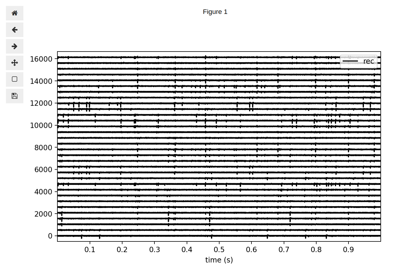
# matplotlib backend
w = plot_traces(recording=recording, backend="matplotlib")
Output:
ipywidgets
The plot_*(..., backend="ipywidgets") functions are only available in Jupyter notebooks or JupyterLab after
calling the %matplotlib widget magic line.
Each function has the following additional arguments:
width_cm: Width of the figure in cm (default 10)
height_cm: Height of the figure in cm (default 6)
display: If True, widgets are immediately displayed
from spikeinterface.preprocessing import common_reference
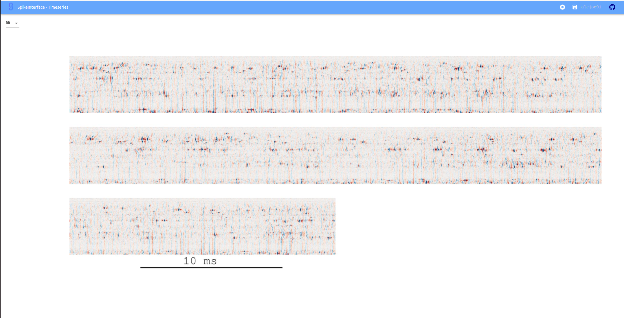
# ipywidgets backend also supports multiple "layers" for plot_traces
rec_dict = dict(filt=recording, cmr=common_reference(recording))
w = sw.plot_traces(recording=rec_dict, backend="ipywidgets")
Output:
sortingview
The plot_*(..., backend="sortingview") generate web-based GUIs, which are also shareable with a link (provided
that kachery-cloud is correctly setup, see Install sortingview).
The functions has the following additional arguments:
generate_url: If True, the figurl URL is generated and printed. Default True
display: If True and in jupyter notebook/lab, the widget is displayed in the cell. Default True
figlabel: The figurl figure label. Default None
height: The height of the sortingview View in jupyter. Default None
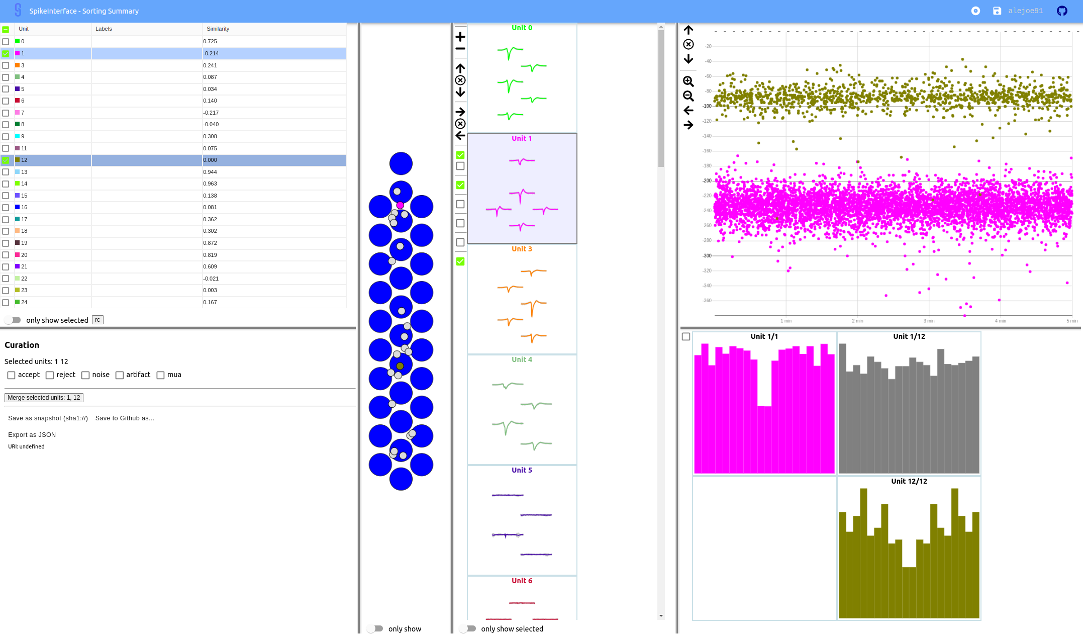
# sortingview backend
w_ts = sw.plot_traces(recording=recording, backend="sortingview")
w_ss = sw.plot_sorting_summary(sorting_analyzer=sorting_analyzer, curation=True, backend="sortingview")
Output:
The sortingview plotter allows one to combine multiple View`s using the :code:`sortingview API.
For example, here is how to combine the timeseries and sorting summary generated above in multiple tabs:
import sortingview.views as vv

v_ts = w_ts.view
v_ss = w_ss.ciew

v_summary = vv.TabLayout(
                items=[
                    vv.TabLayoutItem(
                        label='Timeseries',
                        view=v_ts
                    ),
                    vv.TabLayoutItem(
                        label='Sorting Summary',
                        view=v_ss
                    )
                ]
            )
# generate URL
url = v_summary.url(label="Example multiple tabs")
print(url)
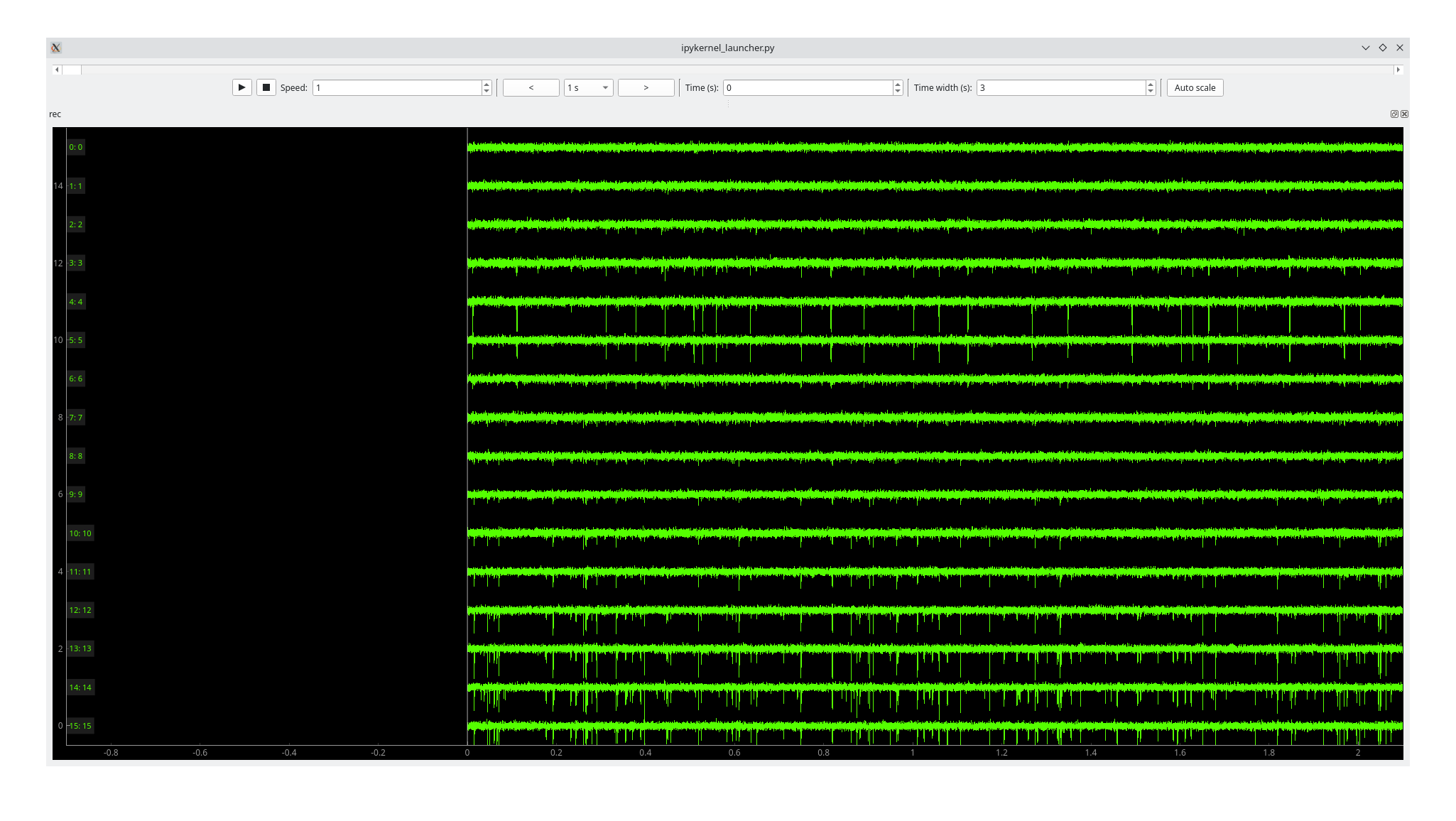
ephyviewer
The ephyviewer backend is currently only available for the plot_traces() function.
plot_traces(recording=recording, backend="ephyviewer", mode="line", show_channel_ids=True)
Available plotting functions
plot_agreement_matrix()(backends:matplotlib)plot_all_amplitudes_distributions()(backends:matplotlib)plot_amplitudes()(backends:matplotlib,ipywidgets,sortingview)plot_autocorrelograms()(backends:matplotlib,sortingview)plot_confusion_matrix()(backends:matplotlib)plot_comparison_collision_by_similarity()(backends:matplotlib)plot_crosscorrelograms()(backends:matplotlib,sortingview)plot_isi_distribution()(backends:matplotlib)plot_motion()(backends:matplotlib)plot_drift_raster_map()(backends:matplotlib,ipywidgets)plot_multicomparison_agreement()(backends:matplotlib)plot_multicomparison_agreement_by_sorter()(backends:matplotlib)plot_multicomparison_graph()(backends:matplotlib)plot_peak_activity()(backends:matplotlib)plot_probe_map()(backends:matplotlib)plot_quality_metrics()(backends:matplotlib,ipywidgets,sortingview)plot_rasters()(backends:matplotlib,ipywidgets)plot_sorting_summary()(backends:sortingview)plot_spike_amplitudes()(backends:matplotlib,ipywidgets)plot_spike_locations()(backends:matplotlib,ipywidgets)plot_spikes_on_traces()(backends:matplotlib,ipywidgets)plot_template_metrics()(backends:matplotlib,ipywidgets,sortingview)plot_template_similarity()(backends: :matplotlib,sortingview)plot_traces()(backends:matplotlib,ipywidgets,sortingview,ephyviewer)plot_unit_depths()(backends:matplotlib)plot_unit_locations()(backends:matplotlib,ipywidgets,sortingview)plot_unit_presence()(backends:matplotlib)plot_unit_probe_map()(backends:matplotlib)plot_unit_summary()(backends:matplotlib)plot_unit_templates()(backends:matplotlib,ipywidgets,sortingview)plot_unit_waveforms_density_map()(backends:matplotlib)plot_unit_waveforms()(backends:matplotlib,ipywidgets)plot_study_run_times()(backends:matplotlib)plot_study_unit_counts()(backends:matplotlib)plot_study_agreement_matrix()(backends:matplotlib)plot_study_summary()(backends:matplotlib)plot_study_comparison_collision_by_similarity()(backends:matplotlib)