Postprocessing module¶

After spike sorting, we can use the postprocessing module to further post-process the spike sorting output. Most of the post-processing functions require a SortingAnalyzer as input.

ResultExtensions¶

There are several postprocessing tools available, and all of them are implemented as a ResultExtension. All computations on top of a SortingAnalyzer will be saved along side the SortingAnalyzer itself (sub folder, zarr path or sub dict). This workflow is convenient for retrieval of time-consuming computations (such as pca or spike amplitudes) when reloading a SortingAnalyzer.

ResultExtension objects are tightly connected to the parent SortingAnalyzer object, so that operations done on the SortingAnalyzer, such as saving, loading, or selecting units, will be automatically applied to all extensions.

To check what extensions are available for a SortingAnalyzer named sorting_analyzer, you can use:

import spikeinterface as si

available_extension_names = sorting_analyzer.get_load_extension_names()
print(available_extension_names)

["principal_components", "spike_amplitudes"]

In this case, for example, principal components and spike amplitudes have already been computed. To load the extension object you can run:

ext = sorting_analyzer.get_extension("spike_amplitudes")
ext_data = ext.get_data()

Here ext is the extension object (in this case the SpikeAmplitudeCalculator), and ext_data will contain the actual amplitude data. Note that different extensions might have different ways to return the extension. You can use ext.get_data? for documentation.

We can also delete an extension:

sorting_analyzer.delete_extension("spike_amplitudes")

Available postprocessing extensions¶

noise_levels¶

This extension computes the noise level of each channel using the median absolute deviation. As an extension, this expects the Recording as input and the computed values are persistent on disk.

noise = compute_noise_level(recording=recording)

principal_components¶

This extension computes the principal components of the waveforms. There are several modes available:

“by_channel_local” (default): fits one PCA model for each by_channel
“by_channel_global”: fits the same PCA model to all channels (also termed temporal PCA)
“concatenated”: concatenates all channels and fits a PCA model on the concatenated data

If the input WaveformExtractor is sparse, the sparsity is used when computing the PCA. For dense waveforms, sparsity can also be passed as an argument.

pc = sorting_analyzer.compute(input="principal_components",
                         n_components=3,
                         mode="by_channel_local")

For more information, see compute_principal_components()

template_similarity¶

This extension computes the similarity of the templates to each other. This information could be used for automatic merging. Currently, the only available similarity method is the cosine similarity, which is the angle between the high-dimensional flattened template arrays. Note that cosine similarity does not take into account amplitude differences and is not well suited for high-density probes.

similarity = sorting_analyzer.compute(input="template_similarity", method='cosine_similarity')

For more information, see compute_template_similarity()

spike_amplitudes¶

This extension computes the amplitude of each spike as the value of the traces on the extremum channel at the times of each spike.

NOTE: computing spike amplitudes is highly recommended before calculating amplitude-based quality metrics, such as Amplitude cutoff (amplitude_cutoff) and Amplitude median (amplitude_median).

amplitudes = sorting_analyzer.compute(input="spike_amplitudes",
                         peak_sign="neg",
                         outputs="concatenated")

For more information, see compute_spike_amplitudes()

spike_locations¶

This extension estimates the location of each spike in the sorting output. Spike location estimates can be done with center of mass (method="center_of_mass" - fast, but less accurate), a monopolar triangulation (method="monopolar_triangulation" - slow, but more accurate), or with the method of grid convolution (method="grid_convolution")

NOTE: computing spike locations is required to compute Drift metrics (drift_ptp, drift_std, drift_mad).

spike_locations = sorting_analyzer.compute(input="spike_locations",
                         ms_before=0.5,
                         ms_after=0.5,
                         spike_retriever_kwargs=dict(
                            channel_from_template=True,
                            radius_um=50,
                            peak_sign="neg"
                                          ),
                         method="center_of_mass")

For more information, see compute_spike_locations()

unit_locations¶

This extension is similar to the spike_locations, but instead of estimating a location for each spike based on individual waveforms, it calculates at the unit level using templates. The same localization methods (method="center_of_mass" | "monopolar_triangulation" | "grid_convolution") are available.

unit_locations = sorting_analyzer.compute(input="unit_locations", method="monopolar_triangulation")

For more information, see compute_unit_locations()

template_metrics¶

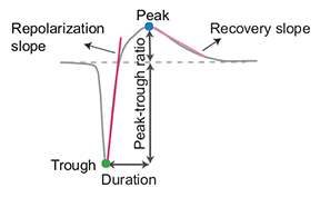
This extension computes commonly used waveform/template metrics. By default, the following metrics are computed:

“peak_to_valley”: duration between negative and positive peaks
“halfwidth”: duration in s at 50% of the amplitude
“peak_to_trough_ratio”: ratio between negative and positive peaks
“recovery_slope”: speed in V/s to recover from the negative peak to 0
“repolarization_slope”: speed in V/s to repolarize from the positive peak to 0
“num_positive_peaks”: the number of positive peaks
“num_negative_peaks”: the number of negative peaks

Optionally, the following multi-channel metrics can be computed by setting: include_multi_channel_metrics=True

“velocity_above”: the velocity above the max channel of the template
“velocity_below”: the velocity below the max channel of the template
“exp_decay”: the exponential decay of the template amplitude over distance
“spread”: the spread of the template amplitude over distance

../_images/1d_waveform_features.png — Visualization of template metrics. Image from ecephys_spike_sorting from the Allen Institute.¶

For more information, see compute_template_metrics()

correlograms¶

This extension computes correlograms (both auto- and cross-) for spike trains. The computed output is a 3d array with shape (num_units, num_units, num_bins) with all correlograms for each pair of units (diagonals are auto-correlograms).

ccg = sorting_analyzer.compute(input="correlograms",
                        window_ms=50.0,
                        bin_ms=1.0,
                        method="auto")

For more information, see compute_correlograms()

isi_histograms¶

This extension computes the histograms of inter-spike-intervals. The computed output is a 2d array with shape (num_units, num_bins), with the isi histogram of each unit.

isi =  sorting_analyer.compute(input="isi_histograms"
                         window_ms=50.0,
                         bin_ms=1.0,
                         method="auto")

For more information, see compute_isi_histograms()