Comparison module
SpikeInterface has a comparison module, which contains functions and tools to compare
spike trains and templates (useful for tracking units over multiple sessions).
Note
In version 0.102.0 the benchmark part of comparison has moved in the new benchmark
In addition, the comparison module contains advanced benchmarking tools to evaluate
the effects of spike collisions on spike sorting results, and to construct hybrid recordings for comparison.
Spike train comparison
For spike train comparison, there are three use cases:
compare a spike sorting output with a ground-truth dataset
compare the output of two spike sorters (symmetric comparison)
compare the output of multiple spike sorters
1. Comparison with ground truth
A ground-truth dataset can be a paired recording, in which a neuron is recorded both extracellularly and with a patch or juxtacellular electrode (either in vitro or in vivo), or it can be a simulated dataset (in silico) using spiking activity simulators such as MEArec.
The comparison to ground-truth datasets is useful to benchmark spike sorting algorithms.
As an example, the SpikeForest platform benchmarks the performance of several spike sorters on a variety of available ground-truth datasets on a daily basis. For more details see spikeforest notes.
This is the main workflow used to compute performance metrics:
- Given:
i = 1, …, n_gt the list of ground-truth (GT) units
k = 1, …., n_tested the list of tested units from spike sorting output
event_counts_GT[i] the number of spikes for each unit of the GT units
event_counts_ST[k] the number of spikes for each unit of the tested units
Matching firing events
For all pairs of a GT unit and a tested unit we first count how many events are matched within a delta_time tolerance (0.4 ms by default).
This gives a matrix called match_event_count of size (n_gt X n_tested). This is an example of the matrix:
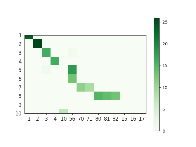
Note that this matrix represents the number of true positive (TP) spikes of each pair. We can also compute the number of false negative (FN) and false positive (FP) spikes.
num_tp [i, k] = match_event_count[i, k]
num_fn [i, k] = event_counts_GT[i] - match_event_count[i, k]
num_fp [i, k] = event_counts_ST[k] - match_event_count[i, k]
Compute agreement score
Given the match_event_count we can then compute the agreement_score, which is normalized to the range [0, 1].
This is done as follows:
agreement_score[i, k] = match_event_count[i, k] / (event_counts_GT[i] + event_counts_ST[k] - match_event_count[i, k])
which is equivalent to:
agreement_score[i, k] = num_tp[i, k] / (num_tp[i, k] + num_fp[i, k] + num_fn[i,k])
or more practically:
agreement_score[i, k] = intersection(I, K) / union(I, K)
which is also equivalent to the accuracy metric.
Here is an example of the agreement matrix, in which only scores > 0.5 are displayed:
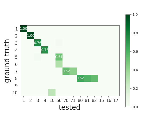
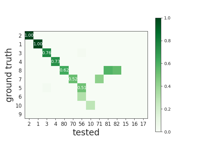
This matrix can be ordered for a better visualization:
Match units
During this step, given the agreement_score matrix each GT unit can be matched to a tested unit. For matching, a minimum match_score is used (0.5 by default). If the agreement is below this threshold, the possible match is discarded.
There are two methods to perform the match: hungarian and best match.
The hungarian method finds the best association between GT and tested units. With this method, both GT and tested units can be matched only to one other unit or are not matched at all.
For the best method, each GT unit is associated to a tested unit that has the best agreement_score, independently of all others units. Using this method several tested units can be associated to the same GT unit. Note that for the “best match” the minimum score is not the match_score, but the chance_score (0.1 by default).
Here is an example of matching with the hungarian method. The first column represents the GT unit id and the second column the tested unit id. -1 means that the tested unit is not matched:
GT    TESTED
0     49
1     -1
2     26
3     44
4     -1
5     35
6     -1
7     -1
8     42
...
Note that the SpikeForest project uses the best match method.
Compute performances
With the list of matched units we can compute performance metrics. Given: tp the number of true positive events, fp number of false positive events, fn the number of false negative events, num_gt the number of events of the matched tested units, the following metrics are computed for each GT unit:
accuracy = tp / (tp + fn + fp)
recall = tp / (tp + fn)
precision = tp / (tp + fp)
false_discovery_rate = fp / (tp + fp)
miss_rate = fn / num_gt
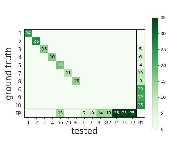
The overall performances can be visualized with the confusion matrix, where the last column contains the FN counts and the last row contains the FP counts.
More information about hungarian or best match methods
Hungarian:
Finds the best pairing. If the matrix is square, then all units are associated. If the matrix is rectangular, then each row is matched. A GT unit (row) can be matched one time only.
Pros
Each spike is counted only once
Hit score near chance levels are set to zero
Good FP estimation
Cons
Does not catch units that are split into several sub-units. Only the best match will be listed
More complicated implementation
Best
Each GT unit is associated to the tested unit that has the best agreement score.
Pros:
Each GT unit is matched totally independently from other units
The accuracy score of a GT unit is totally independent from other units
It can identify over-merged units, as they would match multiple GT units
Cons:
A tested unit can be matched to multiple GT units, so some spikes can be counted several times
FP scores for units associated several times can be biased
Less robust with units having high firing rates
Classification of identified units
Tested units are classified depending on their performance. We identify three different classes:
well-detected units
false positive units
redundant units
over-merged units
A well-detected unit is a unit whose performance is good. By default, a good performance is measured by an accuracy greater than 0.8.
A false positive unit has low agreement scores for all GT units and is not matched.
A redundant unit has a relatively high agreement (>= 0.2 by default), but it is not a best match. This means that it could either be an oversplit unit or a duplicate unit.
An over-merged unit has a relatively high agreement (>= 0.2 by default) for more than one GT unit.
Example: compare one sorter to ground-truth
from spikeinterface.widgets import plot_agreement_matrix, plot_confusion_matrix
from spikeinterface.generation import generate_ground_truth_recording
from spikeinterface.sorters import run_sorter

recording, sorting_true = generate_ground_truth_recording()

# run a sorter and compare to ground truth
sorting_HS = run_sorter(sorter_name='herdingspikes', recording=recording)
cmp_gt_HS = sc.compare_sorter_to_ground_truth(sorting_true, sorting_HS, exhaustive_gt=True)

# To have an overview of the match we can use the ordered agreement matrix
plot_agreement_matrix(cmp_gt_HS, ordered=True)

# This function first matches the ground-truth and spike sorted units, and
# then it computes several performance metrics: accuracy, recall, precision
#
perf = cmp_gt_HS.get_performance()

# The confusion matrix is also a good summary of the score as it has
# the same shape as an agreement matrix, but it contains an extra column for FN
# and an extra row for FP
plot_confusion_matrix(cmp_gt_HS)

# We can query the well and poorly detected units. By default, the threshold
# for accuracy is 0.95.
cmp_gt_HS.get_well_detected_units(well_detected_score=0.95)

cmp_gt_HS.get_false_positive_units(redundant_score=0.2)

cmp_gt_HS.get_redundant_units(redundant_score=0.2)
2. Compare the output of two spike sorters (symmetric comparison)
The comparison of two sorters is quite similar to the procedure of compare to ground truth. The difference is that no assumption is made on which of the units are ground-truth.
So the procedure is the following:
Matching firing events : same as the ground truth comparison
Compute agreement score : same as the ground truth comparison
Match units : only with hungarian method
As there is no ground-truth information, performance metrics are not computed. However, the confusion and agreement matrices can be visualised to assess the level of agreement.
The compare_two_sorters() returns the comparison object to handle this.
Example: compare 2 sorters
import spikeinterface as si
import spikeinterface.sorters as ss
import spikeinterface.comparison as scmp
import spikeinterface.widgets as sw

# First, let's generate a simulated dataset
recording, sorting = si.generate_ground_truth_recording()

# Then run two spike sorters and compare their outputs.
sorting_HS = ss.run_sorter(sorter_name='herdingspikes', recording=recording)
sorting_TDC = ss.run_sorter(sorter_name='tridesclous', recording=recording)

# Run the comparison
# Let's see how to inspect and access this matching.
cmp_HS_TDC = scmp.compare_two_sorters(
    sorting1=sorting_HS,
    sorting2=sorting_TDC,
    sorting1_name='HS',
    sorting2_name='TDC',
)

# We can check the agreement matrix to inspect the matching.
sw.plot_agreement_matrix(sorting_comparison=cmp_HS_TDC)

# Some useful internal dataframes help to check the match and count
# like **match_event_count** or **agreement_scores**
print(cmp_HS_TDC.match_event_count)
print(cmp_HS_TDC.agreement_scores)

# In order to check which units were matched, the `comparison.get_matching()`
# method can be used. If units are not matched they are listed as -1.
sc_to_tdc, tdc_to_sc = cmp_HS_TDC.get_matching()
print('matching HS to TDC')
print(sc_to_tdc)
print('matching TDC to HS')
print(tdc_to_sc)
3. Compare the output of multiple spike sorters
With 3 or more spike sorters, the comparison is implemented with a graph-based method. The multiple sorter comparison also allows cleaning the output by applying a consensus-based method which only selects spike trains and spikes in agreement with multiple sorters.
Comparison of multiple sorters uses the following procedure:
Perform pairwise symmetric comparisons between spike sorters
Construct a graph in which nodes are units and edges are the agreements between units (of different sorters)
Extract units in agreement between two or more spike sorters
Build agreement spike trains, which only contain the spikes in agreement for the comparison with the highest agreement score
Example: compare many sorters
# Generate a simulated dataset
recording, sorting = si.generate_ground_truth_recording()

# Then run 3 spike sorters and compare their outputs.
sorting_MS4 = ss.run_sorter(sorter_name='mountainsort4', recording=recording)
sorting_HS = ss.run_sorter(sorter_name='herdingspikes', recording=recording)
sorting_TDC = ss.run_sorter(sorter_name='tridesclous', recording=recording)

# Compare multiple spike sorter outputs
mcmp = scmp.compare_multiple_sorters(
    sorting_list=[sorting_MS4, sorting_HS, sorting_TDC],
    name_list=['MS4', 'HS', 'TDC'],
    verbose=True,
)

# The multiple sorters comparison internally computes pairwise comparisons,
# that can be accessed as follows:
print(mcmp.comparisons[('MS4', 'HS')].sorting1, mcmp.comparisons[('MS4', 'HS')].sorting2)
print(mcmp.comparisons[('MS4', 'HS')].get_matching())

print(mcmp.comparisons[('MS4', 'TDC')].sorting1, mcmp.comparisons[('MS4', 'TDC')].sorting2)
print(mcmp.comparisons[('MS4', 'TDC')].get_matching())

# The global multi comparison can be visualized with this graph
sw.plot_multicomparison_graph(multi_comparison=mcmp)

# Consensus-based method
#
# We can pull the units in agreement with different sorters using the
# spikeinterface.comparison.MultiSortingComparison.get_agreement_sorting method.
# This allows us to make spike sorting more robust by integrating the outputs of several algorithms.
# On the other hand, it might suffer from weak performances of single algorithms.
# When extracting the units in agreement, the spike trains are modified so
# that only the true positive spikes between the comparison with the best
# match are used.

agr_3 = mcmp.get_agreement_sorting(minimum_agreement_count=3)
print('Units in agreement for all three sorters: ', agr_3.get_unit_ids())

agr_2 = mcmp.get_agreement_sorting(minimum_agreement_count=2)
print('Units in agreement for at least two sorters: ', agr_2.get_unit_ids())

agr_all = mcmp.get_agreement_sorting()

# The unit index of the different sorters can also be retrieved from the
# agreement sorting object (`agr_3`) property `sorter_unit_ids`.

print(agr_3.get_property('unit_ids'))

print(agr_3.get_unit_ids())
# take one unit in agreement
unit_id0 = agr_3.get_unit_ids()[0]
sorter_unit_ids = agr_3.get_property('unit_ids')[0]
print(unit_id0, ':', sorter_unit_ids)
Template comparison
For template comparisons, the underlying ideas are very similar to 2. Compare the output of two spike sorters (symmetric comparison) and 3. Compare the output of multiple spike sorters, for pairwise and multiple comparisons, respectively. In contrast to spike train comparisons, agreement is assessed in the similarity of templates rather than spiking events. This enables us to use exactly the same tools for both types of comparisons, just by changing the way that agreement scores are computed.
The functions to compare templates take a list of SortingAnalyzer objects as input,
which are assumed to be from different sessions of the same animal over time. In this case, let’s assume we have 5
sorting analyzers from day 1 (analyzer_day1) to day 5 (analyzer_day5):
analyzer_list = [analyzer_day1, analyzer_day2, analyzer_day3, analyzer_day4, analyzer_day5]

# match only day 1 and 2
p_tcmp = sc.compare_templates(sorting_analyzer_1=analyzer_day1, sorting_analyzer2=analyzer_day2, name1="Day1", name2="Day2")

# match all
m_tcmp = sc.compare_multiple_templates(waveform_list=analyzer_list,
                                       name_list=["D1", "D2", "D3", "D4", "D5"])