%matplotlib inline
%load_ext autoreload
%autoreload 2
Handle motion/drift in your recording
Spikeinterface offers a very flexible framework to handle drift as a
preprocessing step. If you want to know more, please read the
motion_correction section of the documentation.
Here is a short demo on how to handle drift using the high-level
function spikeinterface.preprocessing.compute_motion().
This function takes a preprocessed recording as input and returns a
motion object, which contains the information required to
interpolate your recording. You can additionally return a
motion_info object which contains the peaks, peak_locations and
parameters used to compute the motion object by passing
output_motion_info = True to the compute_motion function. Note
that you can alternatively compute the motion correction and interpolate
at the same time using the
spikeinterface.preprocessing.correct_motion() function.
Internally the function compute_motion runs the following steps
(which can be slow!):
1. detect_peaks()
2. localize_peaks()
3. select_peaks() (optional)
4. estimate_motion()
All these sub-steps can be run with different methods and have many parameters.
The high-level function suggests several predefined “presets” and we will explore them using a very well known public dataset recorded by Nick Steinmetz: Imposed motion datasets
This dataset contains 3 recordings and each recording contains a Neuropixels 1 and a Neuropixels 2 probe.
Here we will use dataset1 with neuropixel1. This dataset is the “hello world” for drift correction in the spike sorting community!
from pathlib import Path
import matplotlib.pyplot as plt
import numpy as np

import shutil

import spikeinterface.full as si

from spikeinterface.preprocessing import get_motion_parameters_preset, get_motion_presets
/home/nolanlab/Work/Developing/motion_correct_docs/spikeinterface/.venv/lib/python3.13/site-packages/tqdm/auto.py:21: TqdmWarning: IProgress not found. Please update jupyter and ipywidgets. See https://ipywidgets.readthedocs.io/en/stable/user_install.html
  from .autonotebook import tqdm as notebook_tqdm
base_folder = Path("/home/nolanlab/Work/Data")
dataset_folder = base_folder / "dataset1/NP1"
# read the file
raw_rec = si.read_spikeglx(dataset_folder)
raw_rec
Channel IDs
- ['imec0.ap#AP0' 'imec0.ap#AP1' 'imec0.ap#AP2' 'imec0.ap#AP3'
'imec0.ap#AP4' 'imec0.ap#AP5' 'imec0.ap#AP6' 'imec0.ap#AP7'
'imec0.ap#AP8' 'imec0.ap#AP9' 'imec0.ap#AP10' 'imec0.ap#AP11'
'imec0.ap#AP12' 'imec0.ap#AP13' 'imec0.ap#AP14' 'imec0.ap#AP15'
'imec0.ap#AP16' 'imec0.ap#AP17' 'imec0.ap#AP18' 'imec0.ap#AP19'
'imec0.ap#AP20' 'imec0.ap#AP21' 'imec0.ap#AP22' 'imec0.ap#AP23'
'imec0.ap#AP24' 'imec0.ap#AP25' 'imec0.ap#AP26' 'imec0.ap#AP27'
'imec0.ap#AP28' 'imec0.ap#AP29' 'imec0.ap#AP30' 'imec0.ap#AP31'
'imec0.ap#AP32' 'imec0.ap#AP33' 'imec0.ap#AP34' 'imec0.ap#AP35'
'imec0.ap#AP36' 'imec0.ap#AP37' 'imec0.ap#AP38' 'imec0.ap#AP39'
'imec0.ap#AP40' 'imec0.ap#AP41' 'imec0.ap#AP42' 'imec0.ap#AP43'
'imec0.ap#AP44' 'imec0.ap#AP45' 'imec0.ap#AP46' 'imec0.ap#AP47'
'imec0.ap#AP48' 'imec0.ap#AP49' 'imec0.ap#AP50' 'imec0.ap#AP51'
'imec0.ap#AP52' 'imec0.ap#AP53' 'imec0.ap#AP54' 'imec0.ap#AP55'
'imec0.ap#AP56' 'imec0.ap#AP57' 'imec0.ap#AP58' 'imec0.ap#AP59'
'imec0.ap#AP60' 'imec0.ap#AP61' 'imec0.ap#AP62' 'imec0.ap#AP63'
'imec0.ap#AP64' 'imec0.ap#AP65' 'imec0.ap#AP66' 'imec0.ap#AP67'
'imec0.ap#AP68' 'imec0.ap#AP69' 'imec0.ap#AP70' 'imec0.ap#AP71'
'imec0.ap#AP72' 'imec0.ap#AP73' 'imec0.ap#AP74' 'imec0.ap#AP75'
'imec0.ap#AP76' 'imec0.ap#AP77' 'imec0.ap#AP78' 'imec0.ap#AP79'
'imec0.ap#AP80' 'imec0.ap#AP81' 'imec0.ap#AP82' 'imec0.ap#AP83'
'imec0.ap#AP84' 'imec0.ap#AP85' 'imec0.ap#AP86' 'imec0.ap#AP87'
'imec0.ap#AP88' 'imec0.ap#AP89' 'imec0.ap#AP90' 'imec0.ap#AP91'
'imec0.ap#AP92' 'imec0.ap#AP93' 'imec0.ap#AP94' 'imec0.ap#AP95'
'imec0.ap#AP96' 'imec0.ap#AP97' 'imec0.ap#AP98' 'imec0.ap#AP99'
'imec0.ap#AP100' 'imec0.ap#AP101' 'imec0.ap#AP102' 'imec0.ap#AP103'
'imec0.ap#AP104' 'imec0.ap#AP105' 'imec0.ap#AP106' 'imec0.ap#AP107'
'imec0.ap#AP108' 'imec0.ap#AP109' 'imec0.ap#AP110' 'imec0.ap#AP111'
'imec0.ap#AP112' 'imec0.ap#AP113' 'imec0.ap#AP114' 'imec0.ap#AP115'
'imec0.ap#AP116' 'imec0.ap#AP117' 'imec0.ap#AP118' 'imec0.ap#AP119'
'imec0.ap#AP120' 'imec0.ap#AP121' 'imec0.ap#AP122' 'imec0.ap#AP123'
'imec0.ap#AP124' 'imec0.ap#AP125' 'imec0.ap#AP126' 'imec0.ap#AP127'
'imec0.ap#AP128' 'imec0.ap#AP129' 'imec0.ap#AP130' 'imec0.ap#AP131'
'imec0.ap#AP132' 'imec0.ap#AP133' 'imec0.ap#AP134' 'imec0.ap#AP135'
'imec0.ap#AP136' 'imec0.ap#AP137' 'imec0.ap#AP138' 'imec0.ap#AP139'
'imec0.ap#AP140' 'imec0.ap#AP141' 'imec0.ap#AP142' 'imec0.ap#AP143'
'imec0.ap#AP144' 'imec0.ap#AP145' 'imec0.ap#AP146' 'imec0.ap#AP147'
'imec0.ap#AP148' 'imec0.ap#AP149' 'imec0.ap#AP150' 'imec0.ap#AP151'
'imec0.ap#AP152' 'imec0.ap#AP153' 'imec0.ap#AP154' 'imec0.ap#AP155'
'imec0.ap#AP156' 'imec0.ap#AP157' 'imec0.ap#AP158' 'imec0.ap#AP159'
'imec0.ap#AP160' 'imec0.ap#AP161' 'imec0.ap#AP162' 'imec0.ap#AP163'
'imec0.ap#AP164' 'imec0.ap#AP165' 'imec0.ap#AP166' 'imec0.ap#AP167'
'imec0.ap#AP168' 'imec0.ap#AP169' 'imec0.ap#AP170' 'imec0.ap#AP171'
'imec0.ap#AP172' 'imec0.ap#AP173' 'imec0.ap#AP174' 'imec0.ap#AP175'
'imec0.ap#AP176' 'imec0.ap#AP177' 'imec0.ap#AP178' 'imec0.ap#AP179'
'imec0.ap#AP180' 'imec0.ap#AP181' 'imec0.ap#AP182' 'imec0.ap#AP183'
'imec0.ap#AP184' 'imec0.ap#AP185' 'imec0.ap#AP186' 'imec0.ap#AP187'
'imec0.ap#AP188' 'imec0.ap#AP189' 'imec0.ap#AP190' 'imec0.ap#AP191'
'imec0.ap#AP192' 'imec0.ap#AP193' 'imec0.ap#AP194' 'imec0.ap#AP195'
'imec0.ap#AP196' 'imec0.ap#AP197' 'imec0.ap#AP198' 'imec0.ap#AP199'
'imec0.ap#AP200' 'imec0.ap#AP201' 'imec0.ap#AP202' 'imec0.ap#AP203'
'imec0.ap#AP204' 'imec0.ap#AP205' 'imec0.ap#AP206' 'imec0.ap#AP207'
'imec0.ap#AP208' 'imec0.ap#AP209' 'imec0.ap#AP210' 'imec0.ap#AP211'
'imec0.ap#AP212' 'imec0.ap#AP213' 'imec0.ap#AP214' 'imec0.ap#AP215'
'imec0.ap#AP216' 'imec0.ap#AP217' 'imec0.ap#AP218' 'imec0.ap#AP219'
'imec0.ap#AP220' 'imec0.ap#AP221' 'imec0.ap#AP222' 'imec0.ap#AP223'
'imec0.ap#AP224' 'imec0.ap#AP225' 'imec0.ap#AP226' 'imec0.ap#AP227'
'imec0.ap#AP228' 'imec0.ap#AP229' 'imec0.ap#AP230' 'imec0.ap#AP231'
'imec0.ap#AP232' 'imec0.ap#AP233' 'imec0.ap#AP234' 'imec0.ap#AP235'
'imec0.ap#AP236' 'imec0.ap#AP237' 'imec0.ap#AP238' 'imec0.ap#AP239'
'imec0.ap#AP240' 'imec0.ap#AP241' 'imec0.ap#AP242' 'imec0.ap#AP243'
'imec0.ap#AP244' 'imec0.ap#AP245' 'imec0.ap#AP246' 'imec0.ap#AP247'
'imec0.ap#AP248' 'imec0.ap#AP249' 'imec0.ap#AP250' 'imec0.ap#AP251'
'imec0.ap#AP252' 'imec0.ap#AP253' 'imec0.ap#AP254' 'imec0.ap#AP255'
'imec0.ap#AP256' 'imec0.ap#AP257' 'imec0.ap#AP258' 'imec0.ap#AP259'
'imec0.ap#AP260' 'imec0.ap#AP261' 'imec0.ap#AP262' 'imec0.ap#AP263'
'imec0.ap#AP264' 'imec0.ap#AP265' 'imec0.ap#AP266' 'imec0.ap#AP267'
'imec0.ap#AP268' 'imec0.ap#AP269' 'imec0.ap#AP270' 'imec0.ap#AP271'
'imec0.ap#AP272' 'imec0.ap#AP273' 'imec0.ap#AP274' 'imec0.ap#AP275'
'imec0.ap#AP276' 'imec0.ap#AP277' 'imec0.ap#AP278' 'imec0.ap#AP279'
'imec0.ap#AP280' 'imec0.ap#AP281' 'imec0.ap#AP282' 'imec0.ap#AP283'
'imec0.ap#AP284' 'imec0.ap#AP285' 'imec0.ap#AP286' 'imec0.ap#AP287'
'imec0.ap#AP288' 'imec0.ap#AP289' 'imec0.ap#AP290' 'imec0.ap#AP291'
'imec0.ap#AP292' 'imec0.ap#AP293' 'imec0.ap#AP294' 'imec0.ap#AP295'
'imec0.ap#AP296' 'imec0.ap#AP297' 'imec0.ap#AP298' 'imec0.ap#AP299'
'imec0.ap#AP300' 'imec0.ap#AP301' 'imec0.ap#AP302' 'imec0.ap#AP303'
'imec0.ap#AP304' 'imec0.ap#AP305' 'imec0.ap#AP306' 'imec0.ap#AP307'
'imec0.ap#AP308' 'imec0.ap#AP309' 'imec0.ap#AP310' 'imec0.ap#AP311'
'imec0.ap#AP312' 'imec0.ap#AP313' 'imec0.ap#AP314' 'imec0.ap#AP315'
'imec0.ap#AP316' 'imec0.ap#AP317' 'imec0.ap#AP318' 'imec0.ap#AP319'
'imec0.ap#AP320' 'imec0.ap#AP321' 'imec0.ap#AP322' 'imec0.ap#AP323'
'imec0.ap#AP324' 'imec0.ap#AP325' 'imec0.ap#AP326' 'imec0.ap#AP327'
'imec0.ap#AP328' 'imec0.ap#AP329' 'imec0.ap#AP330' 'imec0.ap#AP331'
'imec0.ap#AP332' 'imec0.ap#AP333' 'imec0.ap#AP334' 'imec0.ap#AP335'
'imec0.ap#AP336' 'imec0.ap#AP337' 'imec0.ap#AP338' 'imec0.ap#AP339'
'imec0.ap#AP340' 'imec0.ap#AP341' 'imec0.ap#AP342' 'imec0.ap#AP343'
'imec0.ap#AP344' 'imec0.ap#AP345' 'imec0.ap#AP346' 'imec0.ap#AP347'
'imec0.ap#AP348' 'imec0.ap#AP349' 'imec0.ap#AP350' 'imec0.ap#AP351'
'imec0.ap#AP352' 'imec0.ap#AP353' 'imec0.ap#AP354' 'imec0.ap#AP355'
'imec0.ap#AP356' 'imec0.ap#AP357' 'imec0.ap#AP358' 'imec0.ap#AP359'
'imec0.ap#AP360' 'imec0.ap#AP361' 'imec0.ap#AP362' 'imec0.ap#AP363'
'imec0.ap#AP364' 'imec0.ap#AP365' 'imec0.ap#AP366' 'imec0.ap#AP367'
'imec0.ap#AP368' 'imec0.ap#AP369' 'imec0.ap#AP370' 'imec0.ap#AP371'
'imec0.ap#AP372' 'imec0.ap#AP373' 'imec0.ap#AP374' 'imec0.ap#AP375'
'imec0.ap#AP376' 'imec0.ap#AP377' 'imec0.ap#AP378' 'imec0.ap#AP379'
'imec0.ap#AP380' 'imec0.ap#AP381' 'imec0.ap#AP382' 'imec0.ap#AP383']
Annotations
- is_filtered : False
- probe_0_planar_contour : [[ -11 9989] [ -11 -11] [ 24 -186] [ 59 -11] [ 59 9989]]
- probes_info : [{'model_name': 'Neuropixels 1.0', 'manufacturer': 'IMEC', 'shank_tips': [[24, -186]], 'probe_type': '0', 'serial_number': '18408406612', 'part_number': 'PRB_1_4_0480_1_C', 'port': '1', 'slot': '2'}]
Properties
gain_to_uV
[2.34375 2.34375 2.34375 2.34375 2.34375 2.34375 2.34375 2.34375 2.34375 2.34375 2.34375 2.34375 2.34375 2.34375 2.34375 2.34375 2.34375 2.34375 2.34375 2.34375 2.34375 2.34375 2.34375 2.34375 2.34375 2.34375 2.34375 2.34375 2.34375 2.34375 2.34375 2.34375 2.34375 2.34375 2.34375 2.34375 2.34375 2.34375 2.34375 2.34375 2.34375 2.34375 2.34375 2.34375 2.34375 2.34375 2.34375 2.34375 2.34375 2.34375 2.34375 2.34375 2.34375 2.34375 2.34375 2.34375 2.34375 2.34375 2.34375 2.34375 2.34375 2.34375 2.34375 2.34375 2.34375 2.34375 2.34375 2.34375 2.34375 2.34375 2.34375 2.34375 2.34375 2.34375 2.34375 2.34375 2.34375 2.34375 2.34375 2.34375 2.34375 2.34375 2.34375 2.34375 2.34375 2.34375 2.34375 2.34375 2.34375 2.34375 2.34375 2.34375 2.34375 2.34375 2.34375 2.34375 2.34375 2.34375 2.34375 2.34375 2.34375 2.34375 2.34375 2.34375 2.34375 2.34375 2.34375 2.34375 2.34375 2.34375 2.34375 2.34375 2.34375 2.34375 2.34375 2.34375 2.34375 2.34375 2.34375 2.34375 2.34375 2.34375 2.34375 2.34375 2.34375 2.34375 2.34375 2.34375 2.34375 2.34375 2.34375 2.34375 2.34375 2.34375 2.34375 2.34375 2.34375 2.34375 2.34375 2.34375 2.34375 2.34375 2.34375 2.34375 2.34375 2.34375 2.34375 2.34375 2.34375 2.34375 2.34375 2.34375 2.34375 2.34375 2.34375 2.34375 2.34375 2.34375 2.34375 2.34375 2.34375 2.34375 2.34375 2.34375 2.34375 2.34375 2.34375 2.34375 2.34375 2.34375 2.34375 2.34375 2.34375 2.34375 2.34375 2.34375 2.34375 2.34375 2.34375 2.34375 2.34375 2.34375 2.34375 2.34375 2.34375 2.34375 2.34375 2.34375 2.34375 2.34375 2.34375 2.34375 2.34375 2.34375 2.34375 2.34375 2.34375 2.34375 2.34375 2.34375 2.34375 2.34375 2.34375 2.34375 2.34375 2.34375 2.34375 2.34375 2.34375 2.34375 2.34375 2.34375 2.34375 2.34375 2.34375 2.34375 2.34375 2.34375 2.34375 2.34375 2.34375 2.34375 2.34375 2.34375 2.34375 2.34375 2.34375 2.34375 2.34375 2.34375 2.34375 2.34375 2.34375 2.34375 2.34375 2.34375 2.34375 2.34375 2.34375 2.34375 2.34375 2.34375 2.34375 2.34375 2.34375 2.34375 2.34375 2.34375 2.34375 2.34375 2.34375 2.34375 2.34375 2.34375 2.34375 2.34375 2.34375 2.34375 2.34375 2.34375 2.34375 2.34375 2.34375 2.34375 2.34375 2.34375 2.34375 2.34375 2.34375 2.34375 2.34375 2.34375 2.34375 2.34375 2.34375 2.34375 2.34375 2.34375 2.34375 2.34375 2.34375 2.34375 2.34375 2.34375 2.34375 2.34375 2.34375 2.34375 2.34375 2.34375 2.34375 2.34375 2.34375 2.34375 2.34375 2.34375 2.34375 2.34375 2.34375 2.34375 2.34375 2.34375 2.34375 2.34375 2.34375 2.34375 2.34375 2.34375 2.34375 2.34375 2.34375 2.34375 2.34375 2.34375 2.34375 2.34375 2.34375 2.34375 2.34375 2.34375 2.34375 2.34375 2.34375 2.34375 2.34375 2.34375 2.34375 2.34375 2.34375 2.34375 2.34375 2.34375 2.34375 2.34375 2.34375 2.34375 2.34375 2.34375 2.34375 2.34375 2.34375 2.34375 2.34375 2.34375 2.34375 2.34375 2.34375 2.34375 2.34375 2.34375 2.34375 2.34375 2.34375 2.34375 2.34375 2.34375 2.34375 2.34375 2.34375 2.34375 2.34375 2.34375 2.34375 2.34375 2.34375 2.34375 2.34375 2.34375 2.34375 2.34375 2.34375 2.34375 2.34375 2.34375 2.34375 2.34375 2.34375 2.34375 2.34375 2.34375 2.34375 2.34375 2.34375 2.34375]offset_to_uV
[0. 0. 0. 0. 0. 0. 0. 0. 0. 0. 0. 0. 0. 0. 0. 0. 0. 0. 0. 0. 0. 0. 0. 0. 0. 0. 0. 0. 0. 0. 0. 0. 0. 0. 0. 0. 0. 0. 0. 0. 0. 0. 0. 0. 0. 0. 0. 0. 0. 0. 0. 0. 0. 0. 0. 0. 0. 0. 0. 0. 0. 0. 0. 0. 0. 0. 0. 0. 0. 0. 0. 0. 0. 0. 0. 0. 0. 0. 0. 0. 0. 0. 0. 0. 0. 0. 0. 0. 0. 0. 0. 0. 0. 0. 0. 0. 0. 0. 0. 0. 0. 0. 0. 0. 0. 0. 0. 0. 0. 0. 0. 0. 0. 0. 0. 0. 0. 0. 0. 0. 0. 0. 0. 0. 0. 0. 0. 0. 0. 0. 0. 0. 0. 0. 0. 0. 0. 0. 0. 0. 0. 0. 0. 0. 0. 0. 0. 0. 0. 0. 0. 0. 0. 0. 0. 0. 0. 0. 0. 0. 0. 0. 0. 0. 0. 0. 0. 0. 0. 0. 0. 0. 0. 0. 0. 0. 0. 0. 0. 0. 0. 0. 0. 0. 0. 0. 0. 0. 0. 0. 0. 0. 0. 0. 0. 0. 0. 0. 0. 0. 0. 0. 0. 0. 0. 0. 0. 0. 0. 0. 0. 0. 0. 0. 0. 0. 0. 0. 0. 0. 0. 0. 0. 0. 0. 0. 0. 0. 0. 0. 0. 0. 0. 0. 0. 0. 0. 0. 0. 0. 0. 0. 0. 0. 0. 0. 0. 0. 0. 0. 0. 0. 0. 0. 0. 0. 0. 0. 0. 0. 0. 0. 0. 0. 0. 0. 0. 0. 0. 0. 0. 0. 0. 0. 0. 0. 0. 0. 0. 0. 0. 0. 0. 0. 0. 0. 0. 0. 0. 0. 0. 0. 0. 0. 0. 0. 0. 0. 0. 0. 0. 0. 0. 0. 0. 0. 0. 0. 0. 0. 0. 0. 0. 0. 0. 0. 0. 0. 0. 0. 0. 0. 0. 0. 0. 0. 0. 0. 0. 0. 0. 0. 0. 0. 0. 0. 0. 0. 0. 0. 0. 0. 0. 0. 0. 0. 0. 0. 0. 0. 0. 0. 0. 0. 0. 0. 0. 0. 0. 0. 0. 0. 0. 0. 0. 0. 0. 0. 0. 0. 0. 0. 0. 0. 0. 0. 0. 0. 0. 0. 0. 0. 0. 0.]physical_unit
['uV' 'uV' 'uV' 'uV' 'uV' 'uV' 'uV' 'uV' 'uV' 'uV' 'uV' 'uV' 'uV' 'uV' 'uV' 'uV' 'uV' 'uV' 'uV' 'uV' 'uV' 'uV' 'uV' 'uV' 'uV' 'uV' 'uV' 'uV' 'uV' 'uV' 'uV' 'uV' 'uV' 'uV' 'uV' 'uV' 'uV' 'uV' 'uV' 'uV' 'uV' 'uV' 'uV' 'uV' 'uV' 'uV' 'uV' 'uV' 'uV' 'uV' 'uV' 'uV' 'uV' 'uV' 'uV' 'uV' 'uV' 'uV' 'uV' 'uV' 'uV' 'uV' 'uV' 'uV' 'uV' 'uV' 'uV' 'uV' 'uV' 'uV' 'uV' 'uV' 'uV' 'uV' 'uV' 'uV' 'uV' 'uV' 'uV' 'uV' 'uV' 'uV' 'uV' 'uV' 'uV' 'uV' 'uV' 'uV' 'uV' 'uV' 'uV' 'uV' 'uV' 'uV' 'uV' 'uV' 'uV' 'uV' 'uV' 'uV' 'uV' 'uV' 'uV' 'uV' 'uV' 'uV' 'uV' 'uV' 'uV' 'uV' 'uV' 'uV' 'uV' 'uV' 'uV' 'uV' 'uV' 'uV' 'uV' 'uV' 'uV' 'uV' 'uV' 'uV' 'uV' 'uV' 'uV' 'uV' 'uV' 'uV' 'uV' 'uV' 'uV' 'uV' 'uV' 'uV' 'uV' 'uV' 'uV' 'uV' 'uV' 'uV' 'uV' 'uV' 'uV' 'uV' 'uV' 'uV' 'uV' 'uV' 'uV' 'uV' 'uV' 'uV' 'uV' 'uV' 'uV' 'uV' 'uV' 'uV' 'uV' 'uV' 'uV' 'uV' 'uV' 'uV' 'uV' 'uV' 'uV' 'uV' 'uV' 'uV' 'uV' 'uV' 'uV' 'uV' 'uV' 'uV' 'uV' 'uV' 'uV' 'uV' 'uV' 'uV' 'uV' 'uV' 'uV' 'uV' 'uV' 'uV' 'uV' 'uV' 'uV' 'uV' 'uV' 'uV' 'uV' 'uV' 'uV' 'uV' 'uV' 'uV' 'uV' 'uV' 'uV' 'uV' 'uV' 'uV' 'uV' 'uV' 'uV' 'uV' 'uV' 'uV' 'uV' 'uV' 'uV' 'uV' 'uV' 'uV' 'uV' 'uV' 'uV' 'uV' 'uV' 'uV' 'uV' 'uV' 'uV' 'uV' 'uV' 'uV' 'uV' 'uV' 'uV' 'uV' 'uV' 'uV' 'uV' 'uV' 'uV' 'uV' 'uV' 'uV' 'uV' 'uV' 'uV' 'uV' 'uV' 'uV' 'uV' 'uV' 'uV' 'uV' 'uV' 'uV' 'uV' 'uV' 'uV' 'uV' 'uV' 'uV' 'uV' 'uV' 'uV' 'uV' 'uV' 'uV' 'uV' 'uV' 'uV' 'uV' 'uV' 'uV' 'uV' 'uV' 'uV' 'uV' 'uV' 'uV' 'uV' 'uV' 'uV' 'uV' 'uV' 'uV' 'uV' 'uV' 'uV' 'uV' 'uV' 'uV' 'uV' 'uV' 'uV' 'uV' 'uV' 'uV' 'uV' 'uV' 'uV' 'uV' 'uV' 'uV' 'uV' 'uV' 'uV' 'uV' 'uV' 'uV' 'uV' 'uV' 'uV' 'uV' 'uV' 'uV' 'uV' 'uV' 'uV' 'uV' 'uV' 'uV' 'uV' 'uV' 'uV' 'uV' 'uV' 'uV' 'uV' 'uV' 'uV' 'uV' 'uV' 'uV' 'uV' 'uV' 'uV' 'uV' 'uV' 'uV' 'uV' 'uV' 'uV' 'uV' 'uV' 'uV' 'uV' 'uV' 'uV' 'uV' 'uV' 'uV' 'uV' 'uV' 'uV' 'uV' 'uV' 'uV' 'uV' 'uV' 'uV' 'uV' 'uV' 'uV' 'uV' 'uV' 'uV' 'uV' 'uV' 'uV' 'uV' 'uV' 'uV' 'uV' 'uV' 'uV' 'uV' 'uV' 'uV' 'uV' 'uV' 'uV' 'uV' 'uV']gain_to_physical_unit
[2.34375 2.34375 2.34375 2.34375 2.34375 2.34375 2.34375 2.34375 2.34375 2.34375 2.34375 2.34375 2.34375 2.34375 2.34375 2.34375 2.34375 2.34375 2.34375 2.34375 2.34375 2.34375 2.34375 2.34375 2.34375 2.34375 2.34375 2.34375 2.34375 2.34375 2.34375 2.34375 2.34375 2.34375 2.34375 2.34375 2.34375 2.34375 2.34375 2.34375 2.34375 2.34375 2.34375 2.34375 2.34375 2.34375 2.34375 2.34375 2.34375 2.34375 2.34375 2.34375 2.34375 2.34375 2.34375 2.34375 2.34375 2.34375 2.34375 2.34375 2.34375 2.34375 2.34375 2.34375 2.34375 2.34375 2.34375 2.34375 2.34375 2.34375 2.34375 2.34375 2.34375 2.34375 2.34375 2.34375 2.34375 2.34375 2.34375 2.34375 2.34375 2.34375 2.34375 2.34375 2.34375 2.34375 2.34375 2.34375 2.34375 2.34375 2.34375 2.34375 2.34375 2.34375 2.34375 2.34375 2.34375 2.34375 2.34375 2.34375 2.34375 2.34375 2.34375 2.34375 2.34375 2.34375 2.34375 2.34375 2.34375 2.34375 2.34375 2.34375 2.34375 2.34375 2.34375 2.34375 2.34375 2.34375 2.34375 2.34375 2.34375 2.34375 2.34375 2.34375 2.34375 2.34375 2.34375 2.34375 2.34375 2.34375 2.34375 2.34375 2.34375 2.34375 2.34375 2.34375 2.34375 2.34375 2.34375 2.34375 2.34375 2.34375 2.34375 2.34375 2.34375 2.34375 2.34375 2.34375 2.34375 2.34375 2.34375 2.34375 2.34375 2.34375 2.34375 2.34375 2.34375 2.34375 2.34375 2.34375 2.34375 2.34375 2.34375 2.34375 2.34375 2.34375 2.34375 2.34375 2.34375 2.34375 2.34375 2.34375 2.34375 2.34375 2.34375 2.34375 2.34375 2.34375 2.34375 2.34375 2.34375 2.34375 2.34375 2.34375 2.34375 2.34375 2.34375 2.34375 2.34375 2.34375 2.34375 2.34375 2.34375 2.34375 2.34375 2.34375 2.34375 2.34375 2.34375 2.34375 2.34375 2.34375 2.34375 2.34375 2.34375 2.34375 2.34375 2.34375 2.34375 2.34375 2.34375 2.34375 2.34375 2.34375 2.34375 2.34375 2.34375 2.34375 2.34375 2.34375 2.34375 2.34375 2.34375 2.34375 2.34375 2.34375 2.34375 2.34375 2.34375 2.34375 2.34375 2.34375 2.34375 2.34375 2.34375 2.34375 2.34375 2.34375 2.34375 2.34375 2.34375 2.34375 2.34375 2.34375 2.34375 2.34375 2.34375 2.34375 2.34375 2.34375 2.34375 2.34375 2.34375 2.34375 2.34375 2.34375 2.34375 2.34375 2.34375 2.34375 2.34375 2.34375 2.34375 2.34375 2.34375 2.34375 2.34375 2.34375 2.34375 2.34375 2.34375 2.34375 2.34375 2.34375 2.34375 2.34375 2.34375 2.34375 2.34375 2.34375 2.34375 2.34375 2.34375 2.34375 2.34375 2.34375 2.34375 2.34375 2.34375 2.34375 2.34375 2.34375 2.34375 2.34375 2.34375 2.34375 2.34375 2.34375 2.34375 2.34375 2.34375 2.34375 2.34375 2.34375 2.34375 2.34375 2.34375 2.34375 2.34375 2.34375 2.34375 2.34375 2.34375 2.34375 2.34375 2.34375 2.34375 2.34375 2.34375 2.34375 2.34375 2.34375 2.34375 2.34375 2.34375 2.34375 2.34375 2.34375 2.34375 2.34375 2.34375 2.34375 2.34375 2.34375 2.34375 2.34375 2.34375 2.34375 2.34375 2.34375 2.34375 2.34375 2.34375 2.34375 2.34375 2.34375 2.34375 2.34375 2.34375 2.34375 2.34375 2.34375 2.34375 2.34375 2.34375 2.34375 2.34375 2.34375 2.34375 2.34375 2.34375 2.34375 2.34375 2.34375 2.34375 2.34375 2.34375 2.34375 2.34375 2.34375 2.34375 2.34375 2.34375 2.34375 2.34375 2.34375 2.34375 2.34375 2.34375 2.34375 2.34375 2.34375 2.34375 2.34375]offset_to_physical_unit
[0. 0. 0. 0. 0. 0. 0. 0. 0. 0. 0. 0. 0. 0. 0. 0. 0. 0. 0. 0. 0. 0. 0. 0. 0. 0. 0. 0. 0. 0. 0. 0. 0. 0. 0. 0. 0. 0. 0. 0. 0. 0. 0. 0. 0. 0. 0. 0. 0. 0. 0. 0. 0. 0. 0. 0. 0. 0. 0. 0. 0. 0. 0. 0. 0. 0. 0. 0. 0. 0. 0. 0. 0. 0. 0. 0. 0. 0. 0. 0. 0. 0. 0. 0. 0. 0. 0. 0. 0. 0. 0. 0. 0. 0. 0. 0. 0. 0. 0. 0. 0. 0. 0. 0. 0. 0. 0. 0. 0. 0. 0. 0. 0. 0. 0. 0. 0. 0. 0. 0. 0. 0. 0. 0. 0. 0. 0. 0. 0. 0. 0. 0. 0. 0. 0. 0. 0. 0. 0. 0. 0. 0. 0. 0. 0. 0. 0. 0. 0. 0. 0. 0. 0. 0. 0. 0. 0. 0. 0. 0. 0. 0. 0. 0. 0. 0. 0. 0. 0. 0. 0. 0. 0. 0. 0. 0. 0. 0. 0. 0. 0. 0. 0. 0. 0. 0. 0. 0. 0. 0. 0. 0. 0. 0. 0. 0. 0. 0. 0. 0. 0. 0. 0. 0. 0. 0. 0. 0. 0. 0. 0. 0. 0. 0. 0. 0. 0. 0. 0. 0. 0. 0. 0. 0. 0. 0. 0. 0. 0. 0. 0. 0. 0. 0. 0. 0. 0. 0. 0. 0. 0. 0. 0. 0. 0. 0. 0. 0. 0. 0. 0. 0. 0. 0. 0. 0. 0. 0. 0. 0. 0. 0. 0. 0. 0. 0. 0. 0. 0. 0. 0. 0. 0. 0. 0. 0. 0. 0. 0. 0. 0. 0. 0. 0. 0. 0. 0. 0. 0. 0. 0. 0. 0. 0. 0. 0. 0. 0. 0. 0. 0. 0. 0. 0. 0. 0. 0. 0. 0. 0. 0. 0. 0. 0. 0. 0. 0. 0. 0. 0. 0. 0. 0. 0. 0. 0. 0. 0. 0. 0. 0. 0. 0. 0. 0. 0. 0. 0. 0. 0. 0. 0. 0. 0. 0. 0. 0. 0. 0. 0. 0. 0. 0. 0. 0. 0. 0. 0. 0. 0. 0. 0. 0. 0. 0. 0. 0. 0. 0. 0. 0. 0. 0. 0. 0. 0. 0. 0. 0. 0. 0. 0. 0. 0.]channel_name
['AP0' 'AP1' 'AP2' 'AP3' 'AP4' 'AP5' 'AP6' 'AP7' 'AP8' 'AP9' 'AP10' 'AP11' 'AP12' 'AP13' 'AP14' 'AP15' 'AP16' 'AP17' 'AP18' 'AP19' 'AP20' 'AP21' 'AP22' 'AP23' 'AP24' 'AP25' 'AP26' 'AP27' 'AP28' 'AP29' 'AP30' 'AP31' 'AP32' 'AP33' 'AP34' 'AP35' 'AP36' 'AP37' 'AP38' 'AP39' 'AP40' 'AP41' 'AP42' 'AP43' 'AP44' 'AP45' 'AP46' 'AP47' 'AP48' 'AP49' 'AP50' 'AP51' 'AP52' 'AP53' 'AP54' 'AP55' 'AP56' 'AP57' 'AP58' 'AP59' 'AP60' 'AP61' 'AP62' 'AP63' 'AP64' 'AP65' 'AP66' 'AP67' 'AP68' 'AP69' 'AP70' 'AP71' 'AP72' 'AP73' 'AP74' 'AP75' 'AP76' 'AP77' 'AP78' 'AP79' 'AP80' 'AP81' 'AP82' 'AP83' 'AP84' 'AP85' 'AP86' 'AP87' 'AP88' 'AP89' 'AP90' 'AP91' 'AP92' 'AP93' 'AP94' 'AP95' 'AP96' 'AP97' 'AP98' 'AP99' 'AP100' 'AP101' 'AP102' 'AP103' 'AP104' 'AP105' 'AP106' 'AP107' 'AP108' 'AP109' 'AP110' 'AP111' 'AP112' 'AP113' 'AP114' 'AP115' 'AP116' 'AP117' 'AP118' 'AP119' 'AP120' 'AP121' 'AP122' 'AP123' 'AP124' 'AP125' 'AP126' 'AP127' 'AP128' 'AP129' 'AP130' 'AP131' 'AP132' 'AP133' 'AP134' 'AP135' 'AP136' 'AP137' 'AP138' 'AP139' 'AP140' 'AP141' 'AP142' 'AP143' 'AP144' 'AP145' 'AP146' 'AP147' 'AP148' 'AP149' 'AP150' 'AP151' 'AP152' 'AP153' 'AP154' 'AP155' 'AP156' 'AP157' 'AP158' 'AP159' 'AP160' 'AP161' 'AP162' 'AP163' 'AP164' 'AP165' 'AP166' 'AP167' 'AP168' 'AP169' 'AP170' 'AP171' 'AP172' 'AP173' 'AP174' 'AP175' 'AP176' 'AP177' 'AP178' 'AP179' 'AP180' 'AP181' 'AP182' 'AP183' 'AP184' 'AP185' 'AP186' 'AP187' 'AP188' 'AP189' 'AP190' 'AP191' 'AP192' 'AP193' 'AP194' 'AP195' 'AP196' 'AP197' 'AP198' 'AP199' 'AP200' 'AP201' 'AP202' 'AP203' 'AP204' 'AP205' 'AP206' 'AP207' 'AP208' 'AP209' 'AP210' 'AP211' 'AP212' 'AP213' 'AP214' 'AP215' 'AP216' 'AP217' 'AP218' 'AP219' 'AP220' 'AP221' 'AP222' 'AP223' 'AP224' 'AP225' 'AP226' 'AP227' 'AP228' 'AP229' 'AP230' 'AP231' 'AP232' 'AP233' 'AP234' 'AP235' 'AP236' 'AP237' 'AP238' 'AP239' 'AP240' 'AP241' 'AP242' 'AP243' 'AP244' 'AP245' 'AP246' 'AP247' 'AP248' 'AP249' 'AP250' 'AP251' 'AP252' 'AP253' 'AP254' 'AP255' 'AP256' 'AP257' 'AP258' 'AP259' 'AP260' 'AP261' 'AP262' 'AP263' 'AP264' 'AP265' 'AP266' 'AP267' 'AP268' 'AP269' 'AP270' 'AP271' 'AP272' 'AP273' 'AP274' 'AP275' 'AP276' 'AP277' 'AP278' 'AP279' 'AP280' 'AP281' 'AP282' 'AP283' 'AP284' 'AP285' 'AP286' 'AP287' 'AP288' 'AP289' 'AP290' 'AP291' 'AP292' 'AP293' 'AP294' 'AP295' 'AP296' 'AP297' 'AP298' 'AP299' 'AP300' 'AP301' 'AP302' 'AP303' 'AP304' 'AP305' 'AP306' 'AP307' 'AP308' 'AP309' 'AP310' 'AP311' 'AP312' 'AP313' 'AP314' 'AP315' 'AP316' 'AP317' 'AP318' 'AP319' 'AP320' 'AP321' 'AP322' 'AP323' 'AP324' 'AP325' 'AP326' 'AP327' 'AP328' 'AP329' 'AP330' 'AP331' 'AP332' 'AP333' 'AP334' 'AP335' 'AP336' 'AP337' 'AP338' 'AP339' 'AP340' 'AP341' 'AP342' 'AP343' 'AP344' 'AP345' 'AP346' 'AP347' 'AP348' 'AP349' 'AP350' 'AP351' 'AP352' 'AP353' 'AP354' 'AP355' 'AP356' 'AP357' 'AP358' 'AP359' 'AP360' 'AP361' 'AP362' 'AP363' 'AP364' 'AP365' 'AP366' 'AP367' 'AP368' 'AP369' 'AP370' 'AP371' 'AP372' 'AP373' 'AP374' 'AP375' 'AP376' 'AP377' 'AP378' 'AP379' 'AP380' 'AP381' 'AP382' 'AP383']contact_vector
[(0, 16., 0., 'square', 12., '', 'e0', 0, 'um', 1., 0., 0., 1., 0, 0, 0, 500, 250, 1) (0, 48., 0., 'square', 12., '', 'e1', 1, 'um', 1., 0., 0., 1., 1, 0, 0, 500, 250, 1) (0, 0., 20., 'square', 12., '', 'e2', 2, 'um', 1., 0., 0., 1., 2, 0, 0, 500, 250, 1) (0, 32., 20., 'square', 12., '', 'e3', 3, 'um', 1., 0., 0., 1., 3, 0, 0, 500, 250, 1) (0, 16., 40., 'square', 12., '', 'e4', 4, 'um', 1., 0., 0., 1., 4, 0, 0, 500, 250, 1) (0, 48., 40., 'square', 12., '', 'e5', 5, 'um', 1., 0., 0., 1., 5, 0, 0, 500, 250, 1) (0, 0., 60., 'square', 12., '', 'e6', 6, 'um', 1., 0., 0., 1., 6, 0, 0, 500, 250, 1) (0, 32., 60., 'square', 12., '', 'e7', 7, 'um', 1., 0., 0., 1., 7, 0, 0, 500, 250, 1) (0, 16., 80., 'square', 12., '', 'e8', 8, 'um', 1., 0., 0., 1., 8, 0, 0, 500, 250, 1) (0, 48., 80., 'square', 12., '', 'e9', 9, 'um', 1., 0., 0., 1., 9, 0, 0, 500, 250, 1) (0, 0., 100., 'square', 12., '', 'e10', 10, 'um', 1., 0., 0., 1., 10, 0, 0, 500, 250, 1) (0, 32., 100., 'square', 12., '', 'e11', 11, 'um', 1., 0., 0., 1., 11, 0, 0, 500, 250, 1) (0, 16., 120., 'square', 12., '', 'e12', 12, 'um', 1., 0., 0., 1., 12, 0, 0, 500, 250, 1) (0, 48., 120., 'square', 12., '', 'e13', 13, 'um', 1., 0., 0., 1., 13, 0, 0, 500, 250, 1) (0, 0., 140., 'square', 12., '', 'e14', 14, 'um', 1., 0., 0., 1., 14, 0, 0, 500, 250, 1) (0, 32., 140., 'square', 12., '', 'e15', 15, 'um', 1., 0., 0., 1., 15, 0, 0, 500, 250, 1) (0, 16., 160., 'square', 12., '', 'e16', 16, 'um', 1., 0., 0., 1., 16, 0, 0, 500, 250, 1) (0, 48., 160., 'square', 12., '', 'e17', 17, 'um', 1., 0., 0., 1., 17, 0, 0, 500, 250, 1) (0, 0., 180., 'square', 12., '', 'e18', 18, 'um', 1., 0., 0., 1., 18, 0, 0, 500, 250, 1) (0, 32., 180., 'square', 12., '', 'e19', 19, 'um', 1., 0., 0., 1., 19, 0, 0, 500, 250, 1) (0, 16., 200., 'square', 12., '', 'e20', 20, 'um', 1., 0., 0., 1., 20, 0, 0, 500, 250, 1) (0, 48., 200., 'square', 12., '', 'e21', 21, 'um', 1., 0., 0., 1., 21, 0, 0, 500, 250, 1) (0, 0., 220., 'square', 12., '', 'e22', 22, 'um', 1., 0., 0., 1., 22, 0, 0, 500, 250, 1) (0, 32., 220., 'square', 12., '', 'e23', 23, 'um', 1., 0., 0., 1., 23, 0, 0, 500, 250, 1) (0, 16., 240., 'square', 12., '', 'e24', 24, 'um', 1., 0., 0., 1., 24, 0, 0, 500, 250, 1) (0, 48., 240., 'square', 12., '', 'e25', 25, 'um', 1., 0., 0., 1., 25, 0, 0, 500, 250, 1) (0, 0., 260., 'square', 12., '', 'e26', 26, 'um', 1., 0., 0., 1., 26, 0, 0, 500, 250, 1) (0, 32., 260., 'square', 12., '', 'e27', 27, 'um', 1., 0., 0., 1., 27, 0, 0, 500, 250, 1) (0, 16., 280., 'square', 12., '', 'e28', 28, 'um', 1., 0., 0., 1., 28, 0, 0, 500, 250, 1) (0, 48., 280., 'square', 12., '', 'e29', 29, 'um', 1., 0., 0., 1., 29, 0, 0, 500, 250, 1) (0, 0., 300., 'square', 12., '', 'e30', 30, 'um', 1., 0., 0., 1., 30, 0, 0, 500, 250, 1) (0, 32., 300., 'square', 12., '', 'e31', 31, 'um', 1., 0., 0., 1., 31, 0, 0, 500, 250, 1) (0, 16., 320., 'square', 12., '', 'e32', 32, 'um', 1., 0., 0., 1., 32, 0, 0, 500, 250, 1) (0, 48., 320., 'square', 12., '', 'e33', 33, 'um', 1., 0., 0., 1., 33, 0, 0, 500, 250, 1) (0, 0., 340., 'square', 12., '', 'e34', 34, 'um', 1., 0., 0., 1., 34, 0, 0, 500, 250, 1) (0, 32., 340., 'square', 12., '', 'e35', 35, 'um', 1., 0., 0., 1., 35, 0, 0, 500, 250, 1) (0, 16., 360., 'square', 12., '', 'e36', 36, 'um', 1., 0., 0., 1., 36, 0, 0, 500, 250, 1) (0, 48., 360., 'square', 12., '', 'e37', 37, 'um', 1., 0., 0., 1., 37, 0, 0, 500, 250, 1) (0, 0., 380., 'square', 12., '', 'e38', 38, 'um', 1., 0., 0., 1., 38, 0, 0, 500, 250, 1) (0, 32., 380., 'square', 12., '', 'e39', 39, 'um', 1., 0., 0., 1., 39, 0, 0, 500, 250, 1) (0, 16., 400., 'square', 12., '', 'e40', 40, 'um', 1., 0., 0., 1., 40, 0, 0, 500, 250, 1) (0, 48., 400., 'square', 12., '', 'e41', 41, 'um', 1., 0., 0., 1., 41, 0, 0, 500, 250, 1) (0, 0., 420., 'square', 12., '', 'e42', 42, 'um', 1., 0., 0., 1., 42, 0, 0, 500, 250, 1) (0, 32., 420., 'square', 12., '', 'e43', 43, 'um', 1., 0., 0., 1., 43, 0, 0, 500, 250, 1) (0, 16., 440., 'square', 12., '', 'e44', 44, 'um', 1., 0., 0., 1., 44, 0, 0, 500, 250, 1) (0, 48., 440., 'square', 12., '', 'e45', 45, 'um', 1., 0., 0., 1., 45, 0, 0, 500, 250, 1) (0, 0., 460., 'square', 12., '', 'e46', 46, 'um', 1., 0., 0., 1., 46, 0, 0, 500, 250, 1) (0, 32., 460., 'square', 12., '', 'e47', 47, 'um', 1., 0., 0., 1., 47, 0, 0, 500, 250, 1) (0, 16., 480., 'square', 12., '', 'e48', 48, 'um', 1., 0., 0., 1., 48, 0, 0, 500, 250, 1) (0, 48., 480., 'square', 12., '', 'e49', 49, 'um', 1., 0., 0., 1., 49, 0, 0, 500, 250, 1) (0, 0., 500., 'square', 12., '', 'e50', 50, 'um', 1., 0., 0., 1., 50, 0, 0, 500, 250, 1) (0, 32., 500., 'square', 12., '', 'e51', 51, 'um', 1., 0., 0., 1., 51, 0, 0, 500, 250, 1) (0, 16., 520., 'square', 12., '', 'e52', 52, 'um', 1., 0., 0., 1., 52, 0, 0, 500, 250, 1) (0, 48., 520., 'square', 12., '', 'e53', 53, 'um', 1., 0., 0., 1., 53, 0, 0, 500, 250, 1) (0, 0., 540., 'square', 12., '', 'e54', 54, 'um', 1., 0., 0., 1., 54, 0, 0, 500, 250, 1) (0, 32., 540., 'square', 12., '', 'e55', 55, 'um', 1., 0., 0., 1., 55, 0, 0, 500, 250, 1) (0, 16., 560., 'square', 12., '', 'e56', 56, 'um', 1., 0., 0., 1., 56, 0, 0, 500, 250, 1) (0, 48., 560., 'square', 12., '', 'e57', 57, 'um', 1., 0., 0., 1., 57, 0, 0, 500, 250, 1) (0, 0., 580., 'square', 12., '', 'e58', 58, 'um', 1., 0., 0., 1., 58, 0, 0, 500, 250, 1) (0, 32., 580., 'square', 12., '', 'e59', 59, 'um', 1., 0., 0., 1., 59, 0, 0, 500, 250, 1) (0, 16., 600., 'square', 12., '', 'e60', 60, 'um', 1., 0., 0., 1., 60, 0, 0, 500, 250, 1) (0, 48., 600., 'square', 12., '', 'e61', 61, 'um', 1., 0., 0., 1., 61, 0, 0, 500, 250, 1) (0, 0., 620., 'square', 12., '', 'e62', 62, 'um', 1., 0., 0., 1., 62, 0, 0, 500, 250, 1) (0, 32., 620., 'square', 12., '', 'e63', 63, 'um', 1., 0., 0., 1., 63, 0, 0, 500, 250, 1) (0, 16., 640., 'square', 12., '', 'e64', 64, 'um', 1., 0., 0., 1., 64, 0, 0, 500, 250, 1) (0, 48., 640., 'square', 12., '', 'e65', 65, 'um', 1., 0., 0., 1., 65, 0, 0, 500, 250, 1) (0, 0., 660., 'square', 12., '', 'e66', 66, 'um', 1., 0., 0., 1., 66, 0, 0, 500, 250, 1) (0, 32., 660., 'square', 12., '', 'e67', 67, 'um', 1., 0., 0., 1., 67, 0, 0, 500, 250, 1) (0, 16., 680., 'square', 12., '', 'e68', 68, 'um', 1., 0., 0., 1., 68, 0, 0, 500, 250, 1) (0, 48., 680., 'square', 12., '', 'e69', 69, 'um', 1., 0., 0., 1., 69, 0, 0, 500, 250, 1) (0, 0., 700., 'square', 12., '', 'e70', 70, 'um', 1., 0., 0., 1., 70, 0, 0, 500, 250, 1) (0, 32., 700., 'square', 12., '', 'e71', 71, 'um', 1., 0., 0., 1., 71, 0, 0, 500, 250, 1) (0, 16., 720., 'square', 12., '', 'e72', 72, 'um', 1., 0., 0., 1., 72, 0, 0, 500, 250, 1) (0, 48., 720., 'square', 12., '', 'e73', 73, 'um', 1., 0., 0., 1., 73, 0, 0, 500, 250, 1) (0, 0., 740., 'square', 12., '', 'e74', 74, 'um', 1., 0., 0., 1., 74, 0, 0, 500, 250, 1) (0, 32., 740., 'square', 12., '', 'e75', 75, 'um', 1., 0., 0., 1., 75, 0, 0, 500, 250, 1) (0, 16., 760., 'square', 12., '', 'e76', 76, 'um', 1., 0., 0., 1., 76, 0, 0, 500, 250, 1) (0, 48., 760., 'square', 12., '', 'e77', 77, 'um', 1., 0., 0., 1., 77, 0, 0, 500, 250, 1) (0, 0., 780., 'square', 12., '', 'e78', 78, 'um', 1., 0., 0., 1., 78, 0, 0, 500, 250, 1) (0, 32., 780., 'square', 12., '', 'e79', 79, 'um', 1., 0., 0., 1., 79, 0, 0, 500, 250, 1) (0, 16., 800., 'square', 12., '', 'e80', 80, 'um', 1., 0., 0., 1., 80, 0, 0, 500, 250, 1) (0, 48., 800., 'square', 12., '', 'e81', 81, 'um', 1., 0., 0., 1., 81, 0, 0, 500, 250, 1) (0, 0., 820., 'square', 12., '', 'e82', 82, 'um', 1., 0., 0., 1., 82, 0, 0, 500, 250, 1) (0, 32., 820., 'square', 12., '', 'e83', 83, 'um', 1., 0., 0., 1., 83, 0, 0, 500, 250, 1) (0, 16., 840., 'square', 12., '', 'e84', 84, 'um', 1., 0., 0., 1., 84, 0, 0, 500, 250, 1) (0, 48., 840., 'square', 12., '', 'e85', 85, 'um', 1., 0., 0., 1., 85, 0, 0, 500, 250, 1) (0, 0., 860., 'square', 12., '', 'e86', 86, 'um', 1., 0., 0., 1., 86, 0, 0, 500, 250, 1) (0, 32., 860., 'square', 12., '', 'e87', 87, 'um', 1., 0., 0., 1., 87, 0, 0, 500, 250, 1) (0, 16., 880., 'square', 12., '', 'e88', 88, 'um', 1., 0., 0., 1., 88, 0, 0, 500, 250, 1) (0, 48., 880., 'square', 12., '', 'e89', 89, 'um', 1., 0., 0., 1., 89, 0, 0, 500, 250, 1) (0, 0., 900., 'square', 12., '', 'e90', 90, 'um', 1., 0., 0., 1., 90, 0, 0, 500, 250, 1) (0, 32., 900., 'square', 12., '', 'e91', 91, 'um', 1., 0., 0., 1., 91, 0, 0, 500, 250, 1) (0, 16., 920., 'square', 12., '', 'e92', 92, 'um', 1., 0., 0., 1., 92, 0, 0, 500, 250, 1) (0, 48., 920., 'square', 12., '', 'e93', 93, 'um', 1., 0., 0., 1., 93, 0, 0, 500, 250, 1) (0, 0., 940., 'square', 12., '', 'e94', 94, 'um', 1., 0., 0., 1., 94, 0, 0, 500, 250, 1) (0, 32., 940., 'square', 12., '', 'e95', 95, 'um', 1., 0., 0., 1., 95, 0, 0, 500, 250, 1) (0, 16., 960., 'square', 12., '', 'e96', 96, 'um', 1., 0., 0., 1., 96, 0, 0, 500, 250, 1) (0, 48., 960., 'square', 12., '', 'e97', 97, 'um', 1., 0., 0., 1., 97, 0, 0, 500, 250, 1) (0, 0., 980., 'square', 12., '', 'e98', 98, 'um', 1., 0., 0., 1., 98, 0, 0, 500, 250, 1) (0, 32., 980., 'square', 12., '', 'e99', 99, 'um', 1., 0., 0., 1., 99, 0, 0, 500, 250, 1) (0, 16., 1000., 'square', 12., '', 'e100', 100, 'um', 1., 0., 0., 1., 100, 0, 0, 500, 250, 1) (0, 48., 1000., 'square', 12., '', 'e101', 101, 'um', 1., 0., 0., 1., 101, 0, 0, 500, 250, 1) (0, 0., 1020., 'square', 12., '', 'e102', 102, 'um', 1., 0., 0., 1., 102, 0, 0, 500, 250, 1) (0, 32., 1020., 'square', 12., '', 'e103', 103, 'um', 1., 0., 0., 1., 103, 0, 0, 500, 250, 1) (0, 16., 1040., 'square', 12., '', 'e104', 104, 'um', 1., 0., 0., 1., 104, 0, 0, 500, 250, 1) (0, 48., 1040., 'square', 12., '', 'e105', 105, 'um', 1., 0., 0., 1., 105, 0, 0, 500, 250, 1) (0, 0., 1060., 'square', 12., '', 'e106', 106, 'um', 1., 0., 0., 1., 106, 0, 0, 500, 250, 1) (0, 32., 1060., 'square', 12., '', 'e107', 107, 'um', 1., 0., 0., 1., 107, 0, 0, 500, 250, 1) (0, 16., 1080., 'square', 12., '', 'e108', 108, 'um', 1., 0., 0., 1., 108, 0, 0, 500, 250, 1) (0, 48., 1080., 'square', 12., '', 'e109', 109, 'um', 1., 0., 0., 1., 109, 0, 0, 500, 250, 1) (0, 0., 1100., 'square', 12., '', 'e110', 110, 'um', 1., 0., 0., 1., 110, 0, 0, 500, 250, 1) (0, 32., 1100., 'square', 12., '', 'e111', 111, 'um', 1., 0., 0., 1., 111, 0, 0, 500, 250, 1) (0, 16., 1120., 'square', 12., '', 'e112', 112, 'um', 1., 0., 0., 1., 112, 0, 0, 500, 250, 1) (0, 48., 1120., 'square', 12., '', 'e113', 113, 'um', 1., 0., 0., 1., 113, 0, 0, 500, 250, 1) (0, 0., 1140., 'square', 12., '', 'e114', 114, 'um', 1., 0., 0., 1., 114, 0, 0, 500, 250, 1) (0, 32., 1140., 'square', 12., '', 'e115', 115, 'um', 1., 0., 0., 1., 115, 0, 0, 500, 250, 1) (0, 16., 1160., 'square', 12., '', 'e116', 116, 'um', 1., 0., 0., 1., 116, 0, 0, 500, 250, 1) (0, 48., 1160., 'square', 12., '', 'e117', 117, 'um', 1., 0., 0., 1., 117, 0, 0, 500, 250, 1) (0, 0., 1180., 'square', 12., '', 'e118', 118, 'um', 1., 0., 0., 1., 118, 0, 0, 500, 250, 1) (0, 32., 1180., 'square', 12., '', 'e119', 119, 'um', 1., 0., 0., 1., 119, 0, 0, 500, 250, 1) (0, 16., 1200., 'square', 12., '', 'e120', 120, 'um', 1., 0., 0., 1., 120, 0, 0, 500, 250, 1) (0, 48., 1200., 'square', 12., '', 'e121', 121, 'um', 1., 0., 0., 1., 121, 0, 0, 500, 250, 1) (0, 0., 1220., 'square', 12., '', 'e122', 122, 'um', 1., 0., 0., 1., 122, 0, 0, 500, 250, 1) (0, 32., 1220., 'square', 12., '', 'e123', 123, 'um', 1., 0., 0., 1., 123, 0, 0, 500, 250, 1) (0, 16., 1240., 'square', 12., '', 'e124', 124, 'um', 1., 0., 0., 1., 124, 0, 0, 500, 250, 1) (0, 48., 1240., 'square', 12., '', 'e125', 125, 'um', 1., 0., 0., 1., 125, 0, 0, 500, 250, 1) (0, 0., 1260., 'square', 12., '', 'e126', 126, 'um', 1., 0., 0., 1., 126, 0, 0, 500, 250, 1) (0, 32., 1260., 'square', 12., '', 'e127', 127, 'um', 1., 0., 0., 1., 127, 0, 0, 500, 250, 1) (0, 16., 1280., 'square', 12., '', 'e128', 128, 'um', 1., 0., 0., 1., 128, 0, 0, 500, 250, 1) (0, 48., 1280., 'square', 12., '', 'e129', 129, 'um', 1., 0., 0., 1., 129, 0, 0, 500, 250, 1) (0, 0., 1300., 'square', 12., '', 'e130', 130, 'um', 1., 0., 0., 1., 130, 0, 0, 500, 250, 1) (0, 32., 1300., 'square', 12., '', 'e131', 131, 'um', 1., 0., 0., 1., 131, 0, 0, 500, 250, 1) (0, 16., 1320., 'square', 12., '', 'e132', 132, 'um', 1., 0., 0., 1., 132, 0, 0, 500, 250, 1) (0, 48., 1320., 'square', 12., '', 'e133', 133, 'um', 1., 0., 0., 1., 133, 0, 0, 500, 250, 1) (0, 0., 1340., 'square', 12., '', 'e134', 134, 'um', 1., 0., 0., 1., 134, 0, 0, 500, 250, 1) (0, 32., 1340., 'square', 12., '', 'e135', 135, 'um', 1., 0., 0., 1., 135, 0, 0, 500, 250, 1) (0, 16., 1360., 'square', 12., '', 'e136', 136, 'um', 1., 0., 0., 1., 136, 0, 0, 500, 250, 1) (0, 48., 1360., 'square', 12., '', 'e137', 137, 'um', 1., 0., 0., 1., 137, 0, 0, 500, 250, 1) (0, 0., 1380., 'square', 12., '', 'e138', 138, 'um', 1., 0., 0., 1., 138, 0, 0, 500, 250, 1) (0, 32., 1380., 'square', 12., '', 'e139', 139, 'um', 1., 0., 0., 1., 139, 0, 0, 500, 250, 1) (0, 16., 1400., 'square', 12., '', 'e140', 140, 'um', 1., 0., 0., 1., 140, 0, 0, 500, 250, 1) (0, 48., 1400., 'square', 12., '', 'e141', 141, 'um', 1., 0., 0., 1., 141, 0, 0, 500, 250, 1) (0, 0., 1420., 'square', 12., '', 'e142', 142, 'um', 1., 0., 0., 1., 142, 0, 0, 500, 250, 1) (0, 32., 1420., 'square', 12., '', 'e143', 143, 'um', 1., 0., 0., 1., 143, 0, 0, 500, 250, 1) (0, 16., 1440., 'square', 12., '', 'e144', 144, 'um', 1., 0., 0., 1., 144, 0, 0, 500, 250, 1) (0, 48., 1440., 'square', 12., '', 'e145', 145, 'um', 1., 0., 0., 1., 145, 0, 0, 500, 250, 1) (0, 0., 1460., 'square', 12., '', 'e146', 146, 'um', 1., 0., 0., 1., 146, 0, 0, 500, 250, 1) (0, 32., 1460., 'square', 12., '', 'e147', 147, 'um', 1., 0., 0., 1., 147, 0, 0, 500, 250, 1) (0, 16., 1480., 'square', 12., '', 'e148', 148, 'um', 1., 0., 0., 1., 148, 0, 0, 500, 250, 1) (0, 48., 1480., 'square', 12., '', 'e149', 149, 'um', 1., 0., 0., 1., 149, 0, 0, 500, 250, 1) (0, 0., 1500., 'square', 12., '', 'e150', 150, 'um', 1., 0., 0., 1., 150, 0, 0, 500, 250, 1) (0, 32., 1500., 'square', 12., '', 'e151', 151, 'um', 1., 0., 0., 1., 151, 0, 0, 500, 250, 1) (0, 16., 1520., 'square', 12., '', 'e152', 152, 'um', 1., 0., 0., 1., 152, 0, 0, 500, 250, 1) (0, 48., 1520., 'square', 12., '', 'e153', 153, 'um', 1., 0., 0., 1., 153, 0, 0, 500, 250, 1) (0, 0., 1540., 'square', 12., '', 'e154', 154, 'um', 1., 0., 0., 1., 154, 0, 0, 500, 250, 1) (0, 32., 1540., 'square', 12., '', 'e155', 155, 'um', 1., 0., 0., 1., 155, 0, 0, 500, 250, 1) (0, 16., 1560., 'square', 12., '', 'e156', 156, 'um', 1., 0., 0., 1., 156, 0, 0, 500, 250, 1) (0, 48., 1560., 'square', 12., '', 'e157', 157, 'um', 1., 0., 0., 1., 157, 0, 0, 500, 250, 1) (0, 0., 1580., 'square', 12., '', 'e158', 158, 'um', 1., 0., 0., 1., 158, 0, 0, 500, 250, 1) (0, 32., 1580., 'square', 12., '', 'e159', 159, 'um', 1., 0., 0., 1., 159, 0, 0, 500, 250, 1) (0, 16., 1600., 'square', 12., '', 'e160', 160, 'um', 1., 0., 0., 1., 160, 0, 0, 500, 250, 1) (0, 48., 1600., 'square', 12., '', 'e161', 161, 'um', 1., 0., 0., 1., 161, 0, 0, 500, 250, 1) (0, 0., 1620., 'square', 12., '', 'e162', 162, 'um', 1., 0., 0., 1., 162, 0, 0, 500, 250, 1) (0, 32., 1620., 'square', 12., '', 'e163', 163, 'um', 1., 0., 0., 1., 163, 0, 0, 500, 250, 1) (0, 16., 1640., 'square', 12., '', 'e164', 164, 'um', 1., 0., 0., 1., 164, 0, 0, 500, 250, 1) (0, 48., 1640., 'square', 12., '', 'e165', 165, 'um', 1., 0., 0., 1., 165, 0, 0, 500, 250, 1) (0, 0., 1660., 'square', 12., '', 'e166', 166, 'um', 1., 0., 0., 1., 166, 0, 0, 500, 250, 1) (0, 32., 1660., 'square', 12., '', 'e167', 167, 'um', 1., 0., 0., 1., 167, 0, 0, 500, 250, 1) (0, 16., 1680., 'square', 12., '', 'e168', 168, 'um', 1., 0., 0., 1., 168, 0, 0, 500, 250, 1) (0, 48., 1680., 'square', 12., '', 'e169', 169, 'um', 1., 0., 0., 1., 169, 0, 0, 500, 250, 1) (0, 0., 1700., 'square', 12., '', 'e170', 170, 'um', 1., 0., 0., 1., 170, 0, 0, 500, 250, 1) (0, 32., 1700., 'square', 12., '', 'e171', 171, 'um', 1., 0., 0., 1., 171, 0, 0, 500, 250, 1) (0, 16., 1720., 'square', 12., '', 'e172', 172, 'um', 1., 0., 0., 1., 172, 0, 0, 500, 250, 1) (0, 48., 1720., 'square', 12., '', 'e173', 173, 'um', 1., 0., 0., 1., 173, 0, 0, 500, 250, 1) (0, 0., 1740., 'square', 12., '', 'e174', 174, 'um', 1., 0., 0., 1., 174, 0, 0, 500, 250, 1) (0, 32., 1740., 'square', 12., '', 'e175', 175, 'um', 1., 0., 0., 1., 175, 0, 0, 500, 250, 1) (0, 16., 1760., 'square', 12., '', 'e176', 176, 'um', 1., 0., 0., 1., 176, 0, 0, 500, 250, 1) (0, 48., 1760., 'square', 12., '', 'e177', 177, 'um', 1., 0., 0., 1., 177, 0, 0, 500, 250, 1) (0, 0., 1780., 'square', 12., '', 'e178', 178, 'um', 1., 0., 0., 1., 178, 0, 0, 500, 250, 1) (0, 32., 1780., 'square', 12., '', 'e179', 179, 'um', 1., 0., 0., 1., 179, 0, 0, 500, 250, 1) (0, 16., 1800., 'square', 12., '', 'e180', 180, 'um', 1., 0., 0., 1., 180, 0, 0, 500, 250, 1) (0, 48., 1800., 'square', 12., '', 'e181', 181, 'um', 1., 0., 0., 1., 181, 0, 0, 500, 250, 1) (0, 0., 1820., 'square', 12., '', 'e182', 182, 'um', 1., 0., 0., 1., 182, 0, 0, 500, 250, 1) (0, 32., 1820., 'square', 12., '', 'e183', 183, 'um', 1., 0., 0., 1., 183, 0, 0, 500, 250, 1) (0, 16., 1840., 'square', 12., '', 'e184', 184, 'um', 1., 0., 0., 1., 184, 0, 0, 500, 250, 1) (0, 48., 1840., 'square', 12., '', 'e185', 185, 'um', 1., 0., 0., 1., 185, 0, 0, 500, 250, 1) (0, 0., 1860., 'square', 12., '', 'e186', 186, 'um', 1., 0., 0., 1., 186, 0, 0, 500, 250, 1) (0, 32., 1860., 'square', 12., '', 'e187', 187, 'um', 1., 0., 0., 1., 187, 0, 0, 500, 250, 1) (0, 16., 1880., 'square', 12., '', 'e188', 188, 'um', 1., 0., 0., 1., 188, 0, 0, 500, 250, 1) (0, 48., 1880., 'square', 12., '', 'e189', 189, 'um', 1., 0., 0., 1., 189, 0, 0, 500, 250, 1) (0, 0., 1900., 'square', 12., '', 'e190', 190, 'um', 1., 0., 0., 1., 190, 0, 0, 500, 250, 1) (0, 32., 1900., 'square', 12., '', 'e191', 191, 'um', 1., 0., 0., 1., 191, 0, 0, 500, 250, 1) (0, 16., 1920., 'square', 12., '', 'e192', 192, 'um', 1., 0., 0., 1., 192, 0, 0, 500, 250, 1) (0, 48., 1920., 'square', 12., '', 'e193', 193, 'um', 1., 0., 0., 1., 193, 0, 0, 500, 250, 1) (0, 0., 1940., 'square', 12., '', 'e194', 194, 'um', 1., 0., 0., 1., 194, 0, 0, 500, 250, 1) (0, 32., 1940., 'square', 12., '', 'e195', 195, 'um', 1., 0., 0., 1., 195, 0, 0, 500, 250, 1) (0, 16., 1960., 'square', 12., '', 'e196', 196, 'um', 1., 0., 0., 1., 196, 0, 0, 500, 250, 1) (0, 48., 1960., 'square', 12., '', 'e197', 197, 'um', 1., 0., 0., 1., 197, 0, 0, 500, 250, 1) (0, 0., 1980., 'square', 12., '', 'e198', 198, 'um', 1., 0., 0., 1., 198, 0, 0, 500, 250, 1) (0, 32., 1980., 'square', 12., '', 'e199', 199, 'um', 1., 0., 0., 1., 199, 0, 0, 500, 250, 1) (0, 16., 2000., 'square', 12., '', 'e200', 200, 'um', 1., 0., 0., 1., 200, 0, 0, 500, 250, 1) (0, 48., 2000., 'square', 12., '', 'e201', 201, 'um', 1., 0., 0., 1., 201, 0, 0, 500, 250, 1) (0, 0., 2020., 'square', 12., '', 'e202', 202, 'um', 1., 0., 0., 1., 202, 0, 0, 500, 250, 1) (0, 32., 2020., 'square', 12., '', 'e203', 203, 'um', 1., 0., 0., 1., 203, 0, 0, 500, 250, 1) (0, 16., 2040., 'square', 12., '', 'e204', 204, 'um', 1., 0., 0., 1., 204, 0, 0, 500, 250, 1) (0, 48., 2040., 'square', 12., '', 'e205', 205, 'um', 1., 0., 0., 1., 205, 0, 0, 500, 250, 1) (0, 0., 2060., 'square', 12., '', 'e206', 206, 'um', 1., 0., 0., 1., 206, 0, 0, 500, 250, 1) (0, 32., 2060., 'square', 12., '', 'e207', 207, 'um', 1., 0., 0., 1., 207, 0, 0, 500, 250, 1) (0, 16., 2080., 'square', 12., '', 'e208', 208, 'um', 1., 0., 0., 1., 208, 0, 0, 500, 250, 1) (0, 48., 2080., 'square', 12., '', 'e209', 209, 'um', 1., 0., 0., 1., 209, 0, 0, 500, 250, 1) (0, 0., 2100., 'square', 12., '', 'e210', 210, 'um', 1., 0., 0., 1., 210, 0, 0, 500, 250, 1) (0, 32., 2100., 'square', 12., '', 'e211', 211, 'um', 1., 0., 0., 1., 211, 0, 0, 500, 250, 1) (0, 16., 2120., 'square', 12., '', 'e212', 212, 'um', 1., 0., 0., 1., 212, 0, 0, 500, 250, 1) (0, 48., 2120., 'square', 12., '', 'e213', 213, 'um', 1., 0., 0., 1., 213, 0, 0, 500, 250, 1) (0, 0., 2140., 'square', 12., '', 'e214', 214, 'um', 1., 0., 0., 1., 214, 0, 0, 500, 250, 1) (0, 32., 2140., 'square', 12., '', 'e215', 215, 'um', 1., 0., 0., 1., 215, 0, 0, 500, 250, 1) (0, 16., 2160., 'square', 12., '', 'e216', 216, 'um', 1., 0., 0., 1., 216, 0, 0, 500, 250, 1) (0, 48., 2160., 'square', 12., '', 'e217', 217, 'um', 1., 0., 0., 1., 217, 0, 0, 500, 250, 1) (0, 0., 2180., 'square', 12., '', 'e218', 218, 'um', 1., 0., 0., 1., 218, 0, 0, 500, 250, 1) (0, 32., 2180., 'square', 12., '', 'e219', 219, 'um', 1., 0., 0., 1., 219, 0, 0, 500, 250, 1) (0, 16., 2200., 'square', 12., '', 'e220', 220, 'um', 1., 0., 0., 1., 220, 0, 0, 500, 250, 1) (0, 48., 2200., 'square', 12., '', 'e221', 221, 'um', 1., 0., 0., 1., 221, 0, 0, 500, 250, 1) (0, 0., 2220., 'square', 12., '', 'e222', 222, 'um', 1., 0., 0., 1., 222, 0, 0, 500, 250, 1) (0, 32., 2220., 'square', 12., '', 'e223', 223, 'um', 1., 0., 0., 1., 223, 0, 0, 500, 250, 1) (0, 16., 2240., 'square', 12., '', 'e224', 224, 'um', 1., 0., 0., 1., 224, 0, 0, 500, 250, 1) (0, 48., 2240., 'square', 12., '', 'e225', 225, 'um', 1., 0., 0., 1., 225, 0, 0, 500, 250, 1) (0, 0., 2260., 'square', 12., '', 'e226', 226, 'um', 1., 0., 0., 1., 226, 0, 0, 500, 250, 1) (0, 32., 2260., 'square', 12., '', 'e227', 227, 'um', 1., 0., 0., 1., 227, 0, 0, 500, 250, 1) (0, 16., 2280., 'square', 12., '', 'e228', 228, 'um', 1., 0., 0., 1., 228, 0, 0, 500, 250, 1) (0, 48., 2280., 'square', 12., '', 'e229', 229, 'um', 1., 0., 0., 1., 229, 0, 0, 500, 250, 1) (0, 0., 2300., 'square', 12., '', 'e230', 230, 'um', 1., 0., 0., 1., 230, 0, 0, 500, 250, 1) (0, 32., 2300., 'square', 12., '', 'e231', 231, 'um', 1., 0., 0., 1., 231, 0, 0, 500, 250, 1) (0, 16., 2320., 'square', 12., '', 'e232', 232, 'um', 1., 0., 0., 1., 232, 0, 0, 500, 250, 1) (0, 48., 2320., 'square', 12., '', 'e233', 233, 'um', 1., 0., 0., 1., 233, 0, 0, 500, 250, 1) (0, 0., 2340., 'square', 12., '', 'e234', 234, 'um', 1., 0., 0., 1., 234, 0, 0, 500, 250, 1) (0, 32., 2340., 'square', 12., '', 'e235', 235, 'um', 1., 0., 0., 1., 235, 0, 0, 500, 250, 1) (0, 16., 2360., 'square', 12., '', 'e236', 236, 'um', 1., 0., 0., 1., 236, 0, 0, 500, 250, 1) (0, 48., 2360., 'square', 12., '', 'e237', 237, 'um', 1., 0., 0., 1., 237, 0, 0, 500, 250, 1) (0, 0., 2380., 'square', 12., '', 'e238', 238, 'um', 1., 0., 0., 1., 238, 0, 0, 500, 250, 1) (0, 32., 2380., 'square', 12., '', 'e239', 239, 'um', 1., 0., 0., 1., 239, 0, 0, 500, 250, 1) (0, 16., 2400., 'square', 12., '', 'e240', 240, 'um', 1., 0., 0., 1., 240, 0, 0, 500, 250, 1) (0, 48., 2400., 'square', 12., '', 'e241', 241, 'um', 1., 0., 0., 1., 241, 0, 0, 500, 250, 1) (0, 0., 2420., 'square', 12., '', 'e242', 242, 'um', 1., 0., 0., 1., 242, 0, 0, 500, 250, 1) (0, 32., 2420., 'square', 12., '', 'e243', 243, 'um', 1., 0., 0., 1., 243, 0, 0, 500, 250, 1) (0, 16., 2440., 'square', 12., '', 'e244', 244, 'um', 1., 0., 0., 1., 244, 0, 0, 500, 250, 1) (0, 48., 2440., 'square', 12., '', 'e245', 245, 'um', 1., 0., 0., 1., 245, 0, 0, 500, 250, 1) (0, 0., 2460., 'square', 12., '', 'e246', 246, 'um', 1., 0., 0., 1., 246, 0, 0, 500, 250, 1) (0, 32., 2460., 'square', 12., '', 'e247', 247, 'um', 1., 0., 0., 1., 247, 0, 0, 500, 250, 1) (0, 16., 2480., 'square', 12., '', 'e248', 248, 'um', 1., 0., 0., 1., 248, 0, 0, 500, 250, 1) (0, 48., 2480., 'square', 12., '', 'e249', 249, 'um', 1., 0., 0., 1., 249, 0, 0, 500, 250, 1) (0, 0., 2500., 'square', 12., '', 'e250', 250, 'um', 1., 0., 0., 1., 250, 0, 0, 500, 250, 1) (0, 32., 2500., 'square', 12., '', 'e251', 251, 'um', 1., 0., 0., 1., 251, 0, 0, 500, 250, 1) (0, 16., 2520., 'square', 12., '', 'e252', 252, 'um', 1., 0., 0., 1., 252, 0, 0, 500, 250, 1) (0, 48., 2520., 'square', 12., '', 'e253', 253, 'um', 1., 0., 0., 1., 253, 0, 0, 500, 250, 1) (0, 0., 2540., 'square', 12., '', 'e254', 254, 'um', 1., 0., 0., 1., 254, 0, 0, 500, 250, 1) (0, 32., 2540., 'square', 12., '', 'e255', 255, 'um', 1., 0., 0., 1., 255, 0, 0, 500, 250, 1) (0, 16., 2560., 'square', 12., '', 'e256', 256, 'um', 1., 0., 0., 1., 256, 0, 0, 500, 250, 1) (0, 48., 2560., 'square', 12., '', 'e257', 257, 'um', 1., 0., 0., 1., 257, 0, 0, 500, 250, 1) (0, 0., 2580., 'square', 12., '', 'e258', 258, 'um', 1., 0., 0., 1., 258, 0, 0, 500, 250, 1) (0, 32., 2580., 'square', 12., '', 'e259', 259, 'um', 1., 0., 0., 1., 259, 0, 0, 500, 250, 1) (0, 16., 2600., 'square', 12., '', 'e260', 260, 'um', 1., 0., 0., 1., 260, 0, 0, 500, 250, 1) (0, 48., 2600., 'square', 12., '', 'e261', 261, 'um', 1., 0., 0., 1., 261, 0, 0, 500, 250, 1) (0, 0., 2620., 'square', 12., '', 'e262', 262, 'um', 1., 0., 0., 1., 262, 0, 0, 500, 250, 1) (0, 32., 2620., 'square', 12., '', 'e263', 263, 'um', 1., 0., 0., 1., 263, 0, 0, 500, 250, 1) (0, 16., 2640., 'square', 12., '', 'e264', 264, 'um', 1., 0., 0., 1., 264, 0, 0, 500, 250, 1) (0, 48., 2640., 'square', 12., '', 'e265', 265, 'um', 1., 0., 0., 1., 265, 0, 0, 500, 250, 1) (0, 0., 2660., 'square', 12., '', 'e266', 266, 'um', 1., 0., 0., 1., 266, 0, 0, 500, 250, 1) (0, 32., 2660., 'square', 12., '', 'e267', 267, 'um', 1., 0., 0., 1., 267, 0, 0, 500, 250, 1) (0, 16., 2680., 'square', 12., '', 'e268', 268, 'um', 1., 0., 0., 1., 268, 0, 0, 500, 250, 1) (0, 48., 2680., 'square', 12., '', 'e269', 269, 'um', 1., 0., 0., 1., 269, 0, 0, 500, 250, 1) (0, 0., 2700., 'square', 12., '', 'e270', 270, 'um', 1., 0., 0., 1., 270, 0, 0, 500, 250, 1) (0, 32., 2700., 'square', 12., '', 'e271', 271, 'um', 1., 0., 0., 1., 271, 0, 0, 500, 250, 1) (0, 16., 2720., 'square', 12., '', 'e272', 272, 'um', 1., 0., 0., 1., 272, 0, 0, 500, 250, 1) (0, 48., 2720., 'square', 12., '', 'e273', 273, 'um', 1., 0., 0., 1., 273, 0, 0, 500, 250, 1) (0, 0., 2740., 'square', 12., '', 'e274', 274, 'um', 1., 0., 0., 1., 274, 0, 0, 500, 250, 1) (0, 32., 2740., 'square', 12., '', 'e275', 275, 'um', 1., 0., 0., 1., 275, 0, 0, 500, 250, 1) (0, 16., 2760., 'square', 12., '', 'e276', 276, 'um', 1., 0., 0., 1., 276, 0, 0, 500, 250, 1) (0, 48., 2760., 'square', 12., '', 'e277', 277, 'um', 1., 0., 0., 1., 277, 0, 0, 500, 250, 1) (0, 0., 2780., 'square', 12., '', 'e278', 278, 'um', 1., 0., 0., 1., 278, 0, 0, 500, 250, 1) (0, 32., 2780., 'square', 12., '', 'e279', 279, 'um', 1., 0., 0., 1., 279, 0, 0, 500, 250, 1) (0, 16., 2800., 'square', 12., '', 'e280', 280, 'um', 1., 0., 0., 1., 280, 0, 0, 500, 250, 1) (0, 48., 2800., 'square', 12., '', 'e281', 281, 'um', 1., 0., 0., 1., 281, 0, 0, 500, 250, 1) (0, 0., 2820., 'square', 12., '', 'e282', 282, 'um', 1., 0., 0., 1., 282, 0, 0, 500, 250, 1) (0, 32., 2820., 'square', 12., '', 'e283', 283, 'um', 1., 0., 0., 1., 283, 0, 0, 500, 250, 1) (0, 16., 2840., 'square', 12., '', 'e284', 284, 'um', 1., 0., 0., 1., 284, 0, 0, 500, 250, 1) (0, 48., 2840., 'square', 12., '', 'e285', 285, 'um', 1., 0., 0., 1., 285, 0, 0, 500, 250, 1) (0, 0., 2860., 'square', 12., '', 'e286', 286, 'um', 1., 0., 0., 1., 286, 0, 0, 500, 250, 1) (0, 32., 2860., 'square', 12., '', 'e287', 287, 'um', 1., 0., 0., 1., 287, 0, 0, 500, 250, 1) (0, 16., 2880., 'square', 12., '', 'e288', 288, 'um', 1., 0., 0., 1., 288, 0, 0, 500, 250, 1) (0, 48., 2880., 'square', 12., '', 'e289', 289, 'um', 1., 0., 0., 1., 289, 0, 0, 500, 250, 1) (0, 0., 2900., 'square', 12., '', 'e290', 290, 'um', 1., 0., 0., 1., 290, 0, 0, 500, 250, 1) (0, 32., 2900., 'square', 12., '', 'e291', 291, 'um', 1., 0., 0., 1., 291, 0, 0, 500, 250, 1) (0, 16., 2920., 'square', 12., '', 'e292', 292, 'um', 1., 0., 0., 1., 292, 0, 0, 500, 250, 1) (0, 48., 2920., 'square', 12., '', 'e293', 293, 'um', 1., 0., 0., 1., 293, 0, 0, 500, 250, 1) (0, 0., 2940., 'square', 12., '', 'e294', 294, 'um', 1., 0., 0., 1., 294, 0, 0, 500, 250, 1) (0, 32., 2940., 'square', 12., '', 'e295', 295, 'um', 1., 0., 0., 1., 295, 0, 0, 500, 250, 1) (0, 16., 2960., 'square', 12., '', 'e296', 296, 'um', 1., 0., 0., 1., 296, 0, 0, 500, 250, 1) (0, 48., 2960., 'square', 12., '', 'e297', 297, 'um', 1., 0., 0., 1., 297, 0, 0, 500, 250, 1) (0, 0., 2980., 'square', 12., '', 'e298', 298, 'um', 1., 0., 0., 1., 298, 0, 0, 500, 250, 1) (0, 32., 2980., 'square', 12., '', 'e299', 299, 'um', 1., 0., 0., 1., 299, 0, 0, 500, 250, 1) (0, 16., 3000., 'square', 12., '', 'e300', 300, 'um', 1., 0., 0., 1., 300, 0, 0, 500, 250, 1) (0, 48., 3000., 'square', 12., '', 'e301', 301, 'um', 1., 0., 0., 1., 301, 0, 0, 500, 250, 1) (0, 0., 3020., 'square', 12., '', 'e302', 302, 'um', 1., 0., 0., 1., 302, 0, 0, 500, 250, 1) (0, 32., 3020., 'square', 12., '', 'e303', 303, 'um', 1., 0., 0., 1., 303, 0, 0, 500, 250, 1) (0, 16., 3040., 'square', 12., '', 'e304', 304, 'um', 1., 0., 0., 1., 304, 0, 0, 500, 250, 1) (0, 48., 3040., 'square', 12., '', 'e305', 305, 'um', 1., 0., 0., 1., 305, 0, 0, 500, 250, 1) (0, 0., 3060., 'square', 12., '', 'e306', 306, 'um', 1., 0., 0., 1., 306, 0, 0, 500, 250, 1) (0, 32., 3060., 'square', 12., '', 'e307', 307, 'um', 1., 0., 0., 1., 307, 0, 0, 500, 250, 1) (0, 16., 3080., 'square', 12., '', 'e308', 308, 'um', 1., 0., 0., 1., 308, 0, 0, 500, 250, 1) (0, 48., 3080., 'square', 12., '', 'e309', 309, 'um', 1., 0., 0., 1., 309, 0, 0, 500, 250, 1) (0, 0., 3100., 'square', 12., '', 'e310', 310, 'um', 1., 0., 0., 1., 310, 0, 0, 500, 250, 1) (0, 32., 3100., 'square', 12., '', 'e311', 311, 'um', 1., 0., 0., 1., 311, 0, 0, 500, 250, 1) (0, 16., 3120., 'square', 12., '', 'e312', 312, 'um', 1., 0., 0., 1., 312, 0, 0, 500, 250, 1) (0, 48., 3120., 'square', 12., '', 'e313', 313, 'um', 1., 0., 0., 1., 313, 0, 0, 500, 250, 1) (0, 0., 3140., 'square', 12., '', 'e314', 314, 'um', 1., 0., 0., 1., 314, 0, 0, 500, 250, 1) (0, 32., 3140., 'square', 12., '', 'e315', 315, 'um', 1., 0., 0., 1., 315, 0, 0, 500, 250, 1) (0, 16., 3160., 'square', 12., '', 'e316', 316, 'um', 1., 0., 0., 1., 316, 0, 0, 500, 250, 1) (0, 48., 3160., 'square', 12., '', 'e317', 317, 'um', 1., 0., 0., 1., 317, 0, 0, 500, 250, 1) (0, 0., 3180., 'square', 12., '', 'e318', 318, 'um', 1., 0., 0., 1., 318, 0, 0, 500, 250, 1) (0, 32., 3180., 'square', 12., '', 'e319', 319, 'um', 1., 0., 0., 1., 319, 0, 0, 500, 250, 1) (0, 16., 3200., 'square', 12., '', 'e320', 320, 'um', 1., 0., 0., 1., 320, 0, 0, 500, 250, 1) (0, 48., 3200., 'square', 12., '', 'e321', 321, 'um', 1., 0., 0., 1., 321, 0, 0, 500, 250, 1) (0, 0., 3220., 'square', 12., '', 'e322', 322, 'um', 1., 0., 0., 1., 322, 0, 0, 500, 250, 1) (0, 32., 3220., 'square', 12., '', 'e323', 323, 'um', 1., 0., 0., 1., 323, 0, 0, 500, 250, 1) (0, 16., 3240., 'square', 12., '', 'e324', 324, 'um', 1., 0., 0., 1., 324, 0, 0, 500, 250, 1) (0, 48., 3240., 'square', 12., '', 'e325', 325, 'um', 1., 0., 0., 1., 325, 0, 0, 500, 250, 1) (0, 0., 3260., 'square', 12., '', 'e326', 326, 'um', 1., 0., 0., 1., 326, 0, 0, 500, 250, 1) (0, 32., 3260., 'square', 12., '', 'e327', 327, 'um', 1., 0., 0., 1., 327, 0, 0, 500, 250, 1) (0, 16., 3280., 'square', 12., '', 'e328', 328, 'um', 1., 0., 0., 1., 328, 0, 0, 500, 250, 1) (0, 48., 3280., 'square', 12., '', 'e329', 329, 'um', 1., 0., 0., 1., 329, 0, 0, 500, 250, 1) (0, 0., 3300., 'square', 12., '', 'e330', 330, 'um', 1., 0., 0., 1., 330, 0, 0, 500, 250, 1) (0, 32., 3300., 'square', 12., '', 'e331', 331, 'um', 1., 0., 0., 1., 331, 0, 0, 500, 250, 1) (0, 16., 3320., 'square', 12., '', 'e332', 332, 'um', 1., 0., 0., 1., 332, 0, 0, 500, 250, 1) (0, 48., 3320., 'square', 12., '', 'e333', 333, 'um', 1., 0., 0., 1., 333, 0, 0, 500, 250, 1) (0, 0., 3340., 'square', 12., '', 'e334', 334, 'um', 1., 0., 0., 1., 334, 0, 0, 500, 250, 1) (0, 32., 3340., 'square', 12., '', 'e335', 335, 'um', 1., 0., 0., 1., 335, 0, 0, 500, 250, 1) (0, 16., 3360., 'square', 12., '', 'e336', 336, 'um', 1., 0., 0., 1., 336, 0, 0, 500, 250, 1) (0, 48., 3360., 'square', 12., '', 'e337', 337, 'um', 1., 0., 0., 1., 337, 0, 0, 500, 250, 1) (0, 0., 3380., 'square', 12., '', 'e338', 338, 'um', 1., 0., 0., 1., 338, 0, 0, 500, 250, 1) (0, 32., 3380., 'square', 12., '', 'e339', 339, 'um', 1., 0., 0., 1., 339, 0, 0, 500, 250, 1) (0, 16., 3400., 'square', 12., '', 'e340', 340, 'um', 1., 0., 0., 1., 340, 0, 0, 500, 250, 1) (0, 48., 3400., 'square', 12., '', 'e341', 341, 'um', 1., 0., 0., 1., 341, 0, 0, 500, 250, 1) (0, 0., 3420., 'square', 12., '', 'e342', 342, 'um', 1., 0., 0., 1., 342, 0, 0, 500, 250, 1) (0, 32., 3420., 'square', 12., '', 'e343', 343, 'um', 1., 0., 0., 1., 343, 0, 0, 500, 250, 1) (0, 16., 3440., 'square', 12., '', 'e344', 344, 'um', 1., 0., 0., 1., 344, 0, 0, 500, 250, 1) (0, 48., 3440., 'square', 12., '', 'e345', 345, 'um', 1., 0., 0., 1., 345, 0, 0, 500, 250, 1) (0, 0., 3460., 'square', 12., '', 'e346', 346, 'um', 1., 0., 0., 1., 346, 0, 0, 500, 250, 1) (0, 32., 3460., 'square', 12., '', 'e347', 347, 'um', 1., 0., 0., 1., 347, 0, 0, 500, 250, 1) (0, 16., 3480., 'square', 12., '', 'e348', 348, 'um', 1., 0., 0., 1., 348, 0, 0, 500, 250, 1) (0, 48., 3480., 'square', 12., '', 'e349', 349, 'um', 1., 0., 0., 1., 349, 0, 0, 500, 250, 1) (0, 0., 3500., 'square', 12., '', 'e350', 350, 'um', 1., 0., 0., 1., 350, 0, 0, 500, 250, 1) (0, 32., 3500., 'square', 12., '', 'e351', 351, 'um', 1., 0., 0., 1., 351, 0, 0, 500, 250, 1) (0, 16., 3520., 'square', 12., '', 'e352', 352, 'um', 1., 0., 0., 1., 352, 0, 0, 500, 250, 1) (0, 48., 3520., 'square', 12., '', 'e353', 353, 'um', 1., 0., 0., 1., 353, 0, 0, 500, 250, 1) (0, 0., 3540., 'square', 12., '', 'e354', 354, 'um', 1., 0., 0., 1., 354, 0, 0, 500, 250, 1) (0, 32., 3540., 'square', 12., '', 'e355', 355, 'um', 1., 0., 0., 1., 355, 0, 0, 500, 250, 1) (0, 16., 3560., 'square', 12., '', 'e356', 356, 'um', 1., 0., 0., 1., 356, 0, 0, 500, 250, 1) (0, 48., 3560., 'square', 12., '', 'e357', 357, 'um', 1., 0., 0., 1., 357, 0, 0, 500, 250, 1) (0, 0., 3580., 'square', 12., '', 'e358', 358, 'um', 1., 0., 0., 1., 358, 0, 0, 500, 250, 1) (0, 32., 3580., 'square', 12., '', 'e359', 359, 'um', 1., 0., 0., 1., 359, 0, 0, 500, 250, 1) (0, 16., 3600., 'square', 12., '', 'e360', 360, 'um', 1., 0., 0., 1., 360, 0, 0, 500, 250, 1) (0, 48., 3600., 'square', 12., '', 'e361', 361, 'um', 1., 0., 0., 1., 361, 0, 0, 500, 250, 1) (0, 0., 3620., 'square', 12., '', 'e362', 362, 'um', 1., 0., 0., 1., 362, 0, 0, 500, 250, 1) (0, 32., 3620., 'square', 12., '', 'e363', 363, 'um', 1., 0., 0., 1., 363, 0, 0, 500, 250, 1) (0, 16., 3640., 'square', 12., '', 'e364', 364, 'um', 1., 0., 0., 1., 364, 0, 0, 500, 250, 1) (0, 48., 3640., 'square', 12., '', 'e365', 365, 'um', 1., 0., 0., 1., 365, 0, 0, 500, 250, 1) (0, 0., 3660., 'square', 12., '', 'e366', 366, 'um', 1., 0., 0., 1., 366, 0, 0, 500, 250, 1) (0, 32., 3660., 'square', 12., '', 'e367', 367, 'um', 1., 0., 0., 1., 367, 0, 0, 500, 250, 1) (0, 16., 3680., 'square', 12., '', 'e368', 368, 'um', 1., 0., 0., 1., 368, 0, 0, 500, 250, 1) (0, 48., 3680., 'square', 12., '', 'e369', 369, 'um', 1., 0., 0., 1., 369, 0, 0, 500, 250, 1) (0, 0., 3700., 'square', 12., '', 'e370', 370, 'um', 1., 0., 0., 1., 370, 0, 0, 500, 250, 1) (0, 32., 3700., 'square', 12., '', 'e371', 371, 'um', 1., 0., 0., 1., 371, 0, 0, 500, 250, 1) (0, 16., 3720., 'square', 12., '', 'e372', 372, 'um', 1., 0., 0., 1., 372, 0, 0, 500, 250, 1) (0, 48., 3720., 'square', 12., '', 'e373', 373, 'um', 1., 0., 0., 1., 373, 0, 0, 500, 250, 1) (0, 0., 3740., 'square', 12., '', 'e374', 374, 'um', 1., 0., 0., 1., 374, 0, 0, 500, 250, 1) (0, 32., 3740., 'square', 12., '', 'e375', 375, 'um', 1., 0., 0., 1., 375, 0, 0, 500, 250, 1) (0, 16., 3760., 'square', 12., '', 'e376', 376, 'um', 1., 0., 0., 1., 376, 0, 0, 500, 250, 1) (0, 48., 3760., 'square', 12., '', 'e377', 377, 'um', 1., 0., 0., 1., 377, 0, 0, 500, 250, 1) (0, 0., 3780., 'square', 12., '', 'e378', 378, 'um', 1., 0., 0., 1., 378, 0, 0, 500, 250, 1) (0, 32., 3780., 'square', 12., '', 'e379', 379, 'um', 1., 0., 0., 1., 379, 0, 0, 500, 250, 1) (0, 16., 3800., 'square', 12., '', 'e380', 380, 'um', 1., 0., 0., 1., 380, 0, 0, 500, 250, 1) (0, 48., 3800., 'square', 12., '', 'e381', 381, 'um', 1., 0., 0., 1., 381, 0, 0, 500, 250, 1) (0, 0., 3820., 'square', 12., '', 'e382', 382, 'um', 1., 0., 0., 1., 382, 0, 0, 500, 250, 1) (0, 32., 3820., 'square', 12., '', 'e383', 383, 'um', 1., 0., 0., 1., 383, 0, 0, 500, 250, 1)]location
[[ 16. 0.] [ 48. 0.] [ 0. 20.] [ 32. 20.] [ 16. 40.] [ 48. 40.] [ 0. 60.] [ 32. 60.] [ 16. 80.] [ 48. 80.] [ 0. 100.] [ 32. 100.] [ 16. 120.] [ 48. 120.] [ 0. 140.] [ 32. 140.] [ 16. 160.] [ 48. 160.] [ 0. 180.] [ 32. 180.] [ 16. 200.] [ 48. 200.] [ 0. 220.] [ 32. 220.] [ 16. 240.] [ 48. 240.] [ 0. 260.] [ 32. 260.] [ 16. 280.] [ 48. 280.] [ 0. 300.] [ 32. 300.] [ 16. 320.] [ 48. 320.] [ 0. 340.] [ 32. 340.] [ 16. 360.] [ 48. 360.] [ 0. 380.] [ 32. 380.] [ 16. 400.] [ 48. 400.] [ 0. 420.] [ 32. 420.] [ 16. 440.] [ 48. 440.] [ 0. 460.] [ 32. 460.] [ 16. 480.] [ 48. 480.] [ 0. 500.] [ 32. 500.] [ 16. 520.] [ 48. 520.] [ 0. 540.] [ 32. 540.] [ 16. 560.] [ 48. 560.] [ 0. 580.] [ 32. 580.] [ 16. 600.] [ 48. 600.] [ 0. 620.] [ 32. 620.] [ 16. 640.] [ 48. 640.] [ 0. 660.] [ 32. 660.] [ 16. 680.] [ 48. 680.] [ 0. 700.] [ 32. 700.] [ 16. 720.] [ 48. 720.] [ 0. 740.] [ 32. 740.] [ 16. 760.] [ 48. 760.] [ 0. 780.] [ 32. 780.] [ 16. 800.] [ 48. 800.] [ 0. 820.] [ 32. 820.] [ 16. 840.] [ 48. 840.] [ 0. 860.] [ 32. 860.] [ 16. 880.] [ 48. 880.] [ 0. 900.] [ 32. 900.] [ 16. 920.] [ 48. 920.] [ 0. 940.] [ 32. 940.] [ 16. 960.] [ 48. 960.] [ 0. 980.] [ 32. 980.] [ 16. 1000.] [ 48. 1000.] [ 0. 1020.] [ 32. 1020.] [ 16. 1040.] [ 48. 1040.] [ 0. 1060.] [ 32. 1060.] [ 16. 1080.] [ 48. 1080.] [ 0. 1100.] [ 32. 1100.] [ 16. 1120.] [ 48. 1120.] [ 0. 1140.] [ 32. 1140.] [ 16. 1160.] [ 48. 1160.] [ 0. 1180.] [ 32. 1180.] [ 16. 1200.] [ 48. 1200.] [ 0. 1220.] [ 32. 1220.] [ 16. 1240.] [ 48. 1240.] [ 0. 1260.] [ 32. 1260.] [ 16. 1280.] [ 48. 1280.] [ 0. 1300.] [ 32. 1300.] [ 16. 1320.] [ 48. 1320.] [ 0. 1340.] [ 32. 1340.] [ 16. 1360.] [ 48. 1360.] [ 0. 1380.] [ 32. 1380.] [ 16. 1400.] [ 48. 1400.] [ 0. 1420.] [ 32. 1420.] [ 16. 1440.] [ 48. 1440.] [ 0. 1460.] [ 32. 1460.] [ 16. 1480.] [ 48. 1480.] [ 0. 1500.] [ 32. 1500.] [ 16. 1520.] [ 48. 1520.] [ 0. 1540.] [ 32. 1540.] [ 16. 1560.] [ 48. 1560.] [ 0. 1580.] [ 32. 1580.] [ 16. 1600.] [ 48. 1600.] [ 0. 1620.] [ 32. 1620.] [ 16. 1640.] [ 48. 1640.] [ 0. 1660.] [ 32. 1660.] [ 16. 1680.] [ 48. 1680.] [ 0. 1700.] [ 32. 1700.] [ 16. 1720.] [ 48. 1720.] [ 0. 1740.] [ 32. 1740.] [ 16. 1760.] [ 48. 1760.] [ 0. 1780.] [ 32. 1780.] [ 16. 1800.] [ 48. 1800.] [ 0. 1820.] [ 32. 1820.] [ 16. 1840.] [ 48. 1840.] [ 0. 1860.] [ 32. 1860.] [ 16. 1880.] [ 48. 1880.] [ 0. 1900.] [ 32. 1900.] [ 16. 1920.] [ 48. 1920.] [ 0. 1940.] [ 32. 1940.] [ 16. 1960.] [ 48. 1960.] [ 0. 1980.] [ 32. 1980.] [ 16. 2000.] [ 48. 2000.] [ 0. 2020.] [ 32. 2020.] [ 16. 2040.] [ 48. 2040.] [ 0. 2060.] [ 32. 2060.] [ 16. 2080.] [ 48. 2080.] [ 0. 2100.] [ 32. 2100.] [ 16. 2120.] [ 48. 2120.] [ 0. 2140.] [ 32. 2140.] [ 16. 2160.] [ 48. 2160.] [ 0. 2180.] [ 32. 2180.] [ 16. 2200.] [ 48. 2200.] [ 0. 2220.] [ 32. 2220.] [ 16. 2240.] [ 48. 2240.] [ 0. 2260.] [ 32. 2260.] [ 16. 2280.] [ 48. 2280.] [ 0. 2300.] [ 32. 2300.] [ 16. 2320.] [ 48. 2320.] [ 0. 2340.] [ 32. 2340.] [ 16. 2360.] [ 48. 2360.] [ 0. 2380.] [ 32. 2380.] [ 16. 2400.] [ 48. 2400.] [ 0. 2420.] [ 32. 2420.] [ 16. 2440.] [ 48. 2440.] [ 0. 2460.] [ 32. 2460.] [ 16. 2480.] [ 48. 2480.] [ 0. 2500.] [ 32. 2500.] [ 16. 2520.] [ 48. 2520.] [ 0. 2540.] [ 32. 2540.] [ 16. 2560.] [ 48. 2560.] [ 0. 2580.] [ 32. 2580.] [ 16. 2600.] [ 48. 2600.] [ 0. 2620.] [ 32. 2620.] [ 16. 2640.] [ 48. 2640.] [ 0. 2660.] [ 32. 2660.] [ 16. 2680.] [ 48. 2680.] [ 0. 2700.] [ 32. 2700.] [ 16. 2720.] [ 48. 2720.] [ 0. 2740.] [ 32. 2740.] [ 16. 2760.] [ 48. 2760.] [ 0. 2780.] [ 32. 2780.] [ 16. 2800.] [ 48. 2800.] [ 0. 2820.] [ 32. 2820.] [ 16. 2840.] [ 48. 2840.] [ 0. 2860.] [ 32. 2860.] [ 16. 2880.] [ 48. 2880.] [ 0. 2900.] [ 32. 2900.] [ 16. 2920.] [ 48. 2920.] [ 0. 2940.] [ 32. 2940.] [ 16. 2960.] [ 48. 2960.] [ 0. 2980.] [ 32. 2980.] [ 16. 3000.] [ 48. 3000.] [ 0. 3020.] [ 32. 3020.] [ 16. 3040.] [ 48. 3040.] [ 0. 3060.] [ 32. 3060.] [ 16. 3080.] [ 48. 3080.] [ 0. 3100.] [ 32. 3100.] [ 16. 3120.] [ 48. 3120.] [ 0. 3140.] [ 32. 3140.] [ 16. 3160.] [ 48. 3160.] [ 0. 3180.] [ 32. 3180.] [ 16. 3200.] [ 48. 3200.] [ 0. 3220.] [ 32. 3220.] [ 16. 3240.] [ 48. 3240.] [ 0. 3260.] [ 32. 3260.] [ 16. 3280.] [ 48. 3280.] [ 0. 3300.] [ 32. 3300.] [ 16. 3320.] [ 48. 3320.] [ 0. 3340.] [ 32. 3340.] [ 16. 3360.] [ 48. 3360.] [ 0. 3380.] [ 32. 3380.] [ 16. 3400.] [ 48. 3400.] [ 0. 3420.] [ 32. 3420.] [ 16. 3440.] [ 48. 3440.] [ 0. 3460.] [ 32. 3460.] [ 16. 3480.] [ 48. 3480.] [ 0. 3500.] [ 32. 3500.] [ 16. 3520.] [ 48. 3520.] [ 0. 3540.] [ 32. 3540.] [ 16. 3560.] [ 48. 3560.] [ 0. 3580.] [ 32. 3580.] [ 16. 3600.] [ 48. 3600.] [ 0. 3620.] [ 32. 3620.] [ 16. 3640.] [ 48. 3640.] [ 0. 3660.] [ 32. 3660.] [ 16. 3680.] [ 48. 3680.] [ 0. 3700.] [ 32. 3700.] [ 16. 3720.] [ 48. 3720.] [ 0. 3740.] [ 32. 3740.] [ 16. 3760.] [ 48. 3760.] [ 0. 3780.] [ 32. 3780.] [ 16. 3800.] [ 48. 3800.] [ 0. 3820.] [ 32. 3820.]]group
[0 0 0 0 0 0 0 0 0 0 0 0 0 0 0 0 0 0 0 0 0 0 0 0 0 0 0 0 0 0 0 0 0 0 0 0 0 0 0 0 0 0 0 0 0 0 0 0 0 0 0 0 0 0 0 0 0 0 0 0 0 0 0 0 0 0 0 0 0 0 0 0 0 0 0 0 0 0 0 0 0 0 0 0 0 0 0 0 0 0 0 0 0 0 0 0 0 0 0 0 0 0 0 0 0 0 0 0 0 0 0 0 0 0 0 0 0 0 0 0 0 0 0 0 0 0 0 0 0 0 0 0 0 0 0 0 0 0 0 0 0 0 0 0 0 0 0 0 0 0 0 0 0 0 0 0 0 0 0 0 0 0 0 0 0 0 0 0 0 0 0 0 0 0 0 0 0 0 0 0 0 0 0 0 0 0 0 0 0 0 0 0 0 0 0 0 0 0 0 0 0 0 0 0 0 0 0 0 0 0 0 0 0 0 0 0 0 0 0 0 0 0 0 0 0 0 0 0 0 0 0 0 0 0 0 0 0 0 0 0 0 0 0 0 0 0 0 0 0 0 0 0 0 0 0 0 0 0 0 0 0 0 0 0 0 0 0 0 0 0 0 0 0 0 0 0 0 0 0 0 0 0 0 0 0 0 0 0 0 0 0 0 0 0 0 0 0 0 0 0 0 0 0 0 0 0 0 0 0 0 0 0 0 0 0 0 0 0 0 0 0 0 0 0 0 0 0 0 0 0 0 0 0 0 0 0 0 0 0 0 0 0 0 0 0 0 0 0 0 0 0 0 0 0 0 0 0 0 0 0 0 0 0 0 0 0 0 0 0 0 0 0 0 0 0 0 0 0 0 0 0 0 0 0]inter_sample_shift
[0. 0. 0.07692308 0.07692308 0.15384615 0.15384615 0.23076923 0.23076923 0.30769231 0.30769231 0.38461538 0.38461538 0.46153846 0.46153846 0.53846154 0.53846154 0.61538462 0.61538462 0.69230769 0.69230769 0.76923077 0.76923077 0.84615385 0.84615385 0. 0. 0.07692308 0.07692308 0.15384615 0.15384615 0.23076923 0.23076923 0.30769231 0.30769231 0.38461538 0.38461538 0.46153846 0.46153846 0.53846154 0.53846154 0.61538462 0.61538462 0.69230769 0.69230769 0.76923077 0.76923077 0.84615385 0.84615385 0. 0. 0.07692308 0.07692308 0.15384615 0.15384615 0.23076923 0.23076923 0.30769231 0.30769231 0.38461538 0.38461538 0.46153846 0.46153846 0.53846154 0.53846154 0.61538462 0.61538462 0.69230769 0.69230769 0.76923077 0.76923077 0.84615385 0.84615385 0. 0. 0.07692308 0.07692308 0.15384615 0.15384615 0.23076923 0.23076923 0.30769231 0.30769231 0.38461538 0.38461538 0.46153846 0.46153846 0.53846154 0.53846154 0.61538462 0.61538462 0.69230769 0.69230769 0.76923077 0.76923077 0.84615385 0.84615385 0. 0. 0.07692308 0.07692308 0.15384615 0.15384615 0.23076923 0.23076923 0.30769231 0.30769231 0.38461538 0.38461538 0.46153846 0.46153846 0.53846154 0.53846154 0.61538462 0.61538462 0.69230769 0.69230769 0.76923077 0.76923077 0.84615385 0.84615385 0. 0. 0.07692308 0.07692308 0.15384615 0.15384615 0.23076923 0.23076923 0.30769231 0.30769231 0.38461538 0.38461538 0.46153846 0.46153846 0.53846154 0.53846154 0.61538462 0.61538462 0.69230769 0.69230769 0.76923077 0.76923077 0.84615385 0.84615385 0. 0. 0.07692308 0.07692308 0.15384615 0.15384615 0.23076923 0.23076923 0.30769231 0.30769231 0.38461538 0.38461538 0.46153846 0.46153846 0.53846154 0.53846154 0.61538462 0.61538462 0.69230769 0.69230769 0.76923077 0.76923077 0.84615385 0.84615385 0. 0. 0.07692308 0.07692308 0.15384615 0.15384615 0.23076923 0.23076923 0.30769231 0.30769231 0.38461538 0.38461538 0.46153846 0.46153846 0.53846154 0.53846154 0.61538462 0.61538462 0.69230769 0.69230769 0.76923077 0.76923077 0.84615385 0.84615385 0. 0. 0.07692308 0.07692308 0.15384615 0.15384615 0.23076923 0.23076923 0.30769231 0.30769231 0.38461538 0.38461538 0.46153846 0.46153846 0.53846154 0.53846154 0.61538462 0.61538462 0.69230769 0.69230769 0.76923077 0.76923077 0.84615385 0.84615385 0. 0. 0.07692308 0.07692308 0.15384615 0.15384615 0.23076923 0.23076923 0.30769231 0.30769231 0.38461538 0.38461538 0.46153846 0.46153846 0.53846154 0.53846154 0.61538462 0.61538462 0.69230769 0.69230769 0.76923077 0.76923077 0.84615385 0.84615385 0. 0. 0.07692308 0.07692308 0.15384615 0.15384615 0.23076923 0.23076923 0.30769231 0.30769231 0.38461538 0.38461538 0.46153846 0.46153846 0.53846154 0.53846154 0.61538462 0.61538462 0.69230769 0.69230769 0.76923077 0.76923077 0.84615385 0.84615385 0. 0. 0.07692308 0.07692308 0.15384615 0.15384615 0.23076923 0.23076923 0.30769231 0.30769231 0.38461538 0.38461538 0.46153846 0.46153846 0.53846154 0.53846154 0.61538462 0.61538462 0.69230769 0.69230769 0.76923077 0.76923077 0.84615385 0.84615385 0. 0. 0.07692308 0.07692308 0.15384615 0.15384615 0.23076923 0.23076923 0.30769231 0.30769231 0.38461538 0.38461538 0.46153846 0.46153846 0.53846154 0.53846154 0.61538462 0.61538462 0.69230769 0.69230769 0.76923077 0.76923077 0.84615385 0.84615385 0. 0. 0.07692308 0.07692308 0.15384615 0.15384615 0.23076923 0.23076923 0.30769231 0.30769231 0.38461538 0.38461538 0.46153846 0.46153846 0.53846154 0.53846154 0.61538462 0.61538462 0.69230769 0.69230769 0.76923077 0.76923077 0.84615385 0.84615385 0. 0. 0.07692308 0.07692308 0.15384615 0.15384615 0.23076923 0.23076923 0.30769231 0.30769231 0.38461538 0.38461538 0.46153846 0.46153846 0.53846154 0.53846154 0.61538462 0.61538462 0.69230769 0.69230769 0.76923077 0.76923077 0.84615385 0.84615385 0. 0. 0.07692308 0.07692308 0.15384615 0.15384615 0.23076923 0.23076923 0.30769231 0.30769231 0.38461538 0.38461538 0.46153846 0.46153846 0.53846154 0.53846154 0.61538462 0.61538462 0.69230769 0.69230769 0.76923077 0.76923077 0.84615385 0.84615385]We preprocess the recording with bandpass filter and a common median reference. Note, that it is better to not whiten the recording before motion estimation to get a better estimate of peak locations!
def preprocess_chain(rec):
    rec = rec.astype('float32')
    rec = si.bandpass_filter(rec, freq_min=300.0, freq_max=6000.0)
    rec = si.common_reference(rec, reference="global", operator="median")
    return rec
rec = preprocess_chain(raw_rec)
job_kwargs = dict(n_jobs=10, chunk_duration="1s", progress_bar=True)
Correcting for drift is easy! You just need to run a single function. We will try this function with some presets.
Internally a preset is a dictionary of dictionaries containing all parameters for every steps.
Here we also save the motion correction results into a folder to be able to load them later.
Preset and parameters
Motion correction has some steps and every step can be controlled by a method and related parameters.
A preset is a nested dict that contains theses methods/parameters.
preset_keys = get_motion_presets()
preset_keys
['dredge',
 'medicine',
 'dredge_fast',
 'nonrigid_accurate',
 'nonrigid_fast_and_accurate',
 'rigid_fast',
 'kilosort_like']
one_preset_params = get_motion_parameters_preset("kilosort_like")
one_preset_params
{'doc': 'Mimic the drift correction of kilosort (grid_convolution + iterative_template)',
 'detect_kwargs': {'peak_sign': 'neg',
  'detect_threshold': 8.0,
  'exclude_sweep_ms': 0.1,
  'radius_um': 50,
  'noise_levels': None,
  'random_chunk_kwargs': {},
  'method': 'locally_exclusive'},
 'select_kwargs': {},
 'localize_peaks_kwargs': {'radius_um': 40.0,
  'upsampling_um': 5.0,
  'sigma_ms': 0.25,
  'margin_um': 50.0,
  'prototype': None,
  'percentile': 5.0,
  'peak_sign': 'neg',
  'weight_method': {'mode': 'gaussian_2d',
   'sigma_list_um': array([ 5., 10., 15., 20., 25.])},
  'method': 'grid_convolution'},
 'estimate_motion_kwargs': {'direction': 'y',
  'rigid': False,
  'win_shape': 'rect',
  'win_step_um': 200.0,
  'win_scale_um': 400.0,
  'win_margin_um': None,
  'bin_um': 10.0,
  'hist_margin_um': 0,
  'bin_s': 2.0,
  'num_amp_bins': 20,
  'num_shifts_global': 15,
  'num_iterations': 10,
  'num_shifts_block': 5,
  'smoothing_sigma': 0.5,
  'kriging_sigma': 1,
  'kriging_p': 2,
  'kriging_d': 2,
  'method': 'iterative_template'},
 'interpolate_motion_kwargs': {'border_mode': 'force_extrapolate',
  'spatial_interpolation_method': 'kriging',
  'sigma_um': 20.0,
  'p': 2}}
Run motion correction with one function!
Here we also save the motion correction results into a folder to be able to load them later.
# lets try theses presets
some_presets = ("rigid_fast", "kilosort_like",  "nonrigid_accurate", "nonrigid_fast_and_accurate", "dredge", "dredge_fast", "medicine")
# compute motion with theses presets
for preset in some_presets:
    print("Computing with", preset)
    folder = base_folder / "motion_folder_dataset1" / preset
    if folder.exists():
        shutil.rmtree(folder)
    motion, motion_info = si.compute_motion(
        rec, preset=preset, folder=folder, output_motion_info=True, **job_kwargs
    )
Computing with rigid_fast
noise_level (no parallelization):   0%|          | 0/20 [00:00<?, ?it/s]noise_level (no parallelization): 100%|██████████| 20/20 [00:04<00:00,  4.09it/s]
detect and localize (workers: 10 processes): 100%|██████████| 1958/1958 [02:48<00:00, 11.63it/s]
/home/nolanlab/Work/Developing/motion_correct_docs/spikeinterface/.venv/lib/python3.13/site-packages/torch/cuda/__init__.py:174: UserWarning: CUDA initialization: Unexpected error from cudaGetDeviceCount(). Did you run some cuda functions before calling NumCudaDevices() that might have already set an error? Error 804: forward compatibility was attempted on non supported HW (Triggered internally at /pytorch/c10/cuda/CUDAFunctions.cpp:109.)
  return torch._C._cuda_getDeviceCount() > 0
Cross correlation: 100%|██████████| 1/1 [00:05<00:00,  5.33s/it]
Computing with kilosort_like
detect and localize (workers: 10 processes): 100%|██████████| 1958/1958 [04:33<00:00, 7.16it/s]
Computing with nonrigid_accurate
detect and localize (workers: 10 processes): 100%|██████████| 1958/1958 [04:47<00:00,  6.82it/s]
pairwise displacement: 100%|██████████| 18/18 [01:01<00:00,  3.43s/it]
Computing with nonrigid_fast_and_accurate
detect and localize (workers: 10 processes): 100%|██████████| 1958/1958 [04:15<00:00,  7.67it/s]
pairwise displacement: 100%|██████████| 18/18 [01:00<00:00,  3.37s/it]
Computing with dredge
detect and localize (workers: 10 processes): 100%|██████████| 1958/1958 [04:45<00:00,  6.87it/s]
Cross correlation: 100%|██████████| 9/9 [01:33<00:00, 10.35s/it]
Solve: 100%|██████████| 8/8 [00:30<00:00,  3.85s/it]
Computing with dredge_fast
detect and localize (workers: 10 processes): 100%|██████████| 1958/1958 [04:13<00:00,  7.72it/s]
Cross correlation: 100%|██████████| 9/9 [01:29<00:00,  9.94s/it]
Solve: 100%|██████████| 8/8 [00:30<00:00,  3.85s/it]
Computing with medicine
detect and localize (workers: 10 processes): 100%|██████████| 1958/1958 [06:52<00:00,  4.75it/s]
[INFO] - Constructing Dataset instance
[INFO] - Constructing MotionFunction instance with parameters:
    bound_normalized = 0.10328739313377586
    time_range = (np.float64(0.0005666666666666667), np.float64(1957.1912))
    time_bin_size = 1.0
    time_kernel_width = 30
    num_depth_bins = 13
[INFO] - Constructing ActivityNetwork instance with parameters:
    hidden_features = (256, 256)
    activation = None
[INFO] - Constructing Medicine instance
num_depth_bins 13
[INFO] - Fitting motion estimation
100%|██████████| 10000/10000 [02:49<00:00, 59.09it/s]
[INFO] - Finished fitting motion estimation
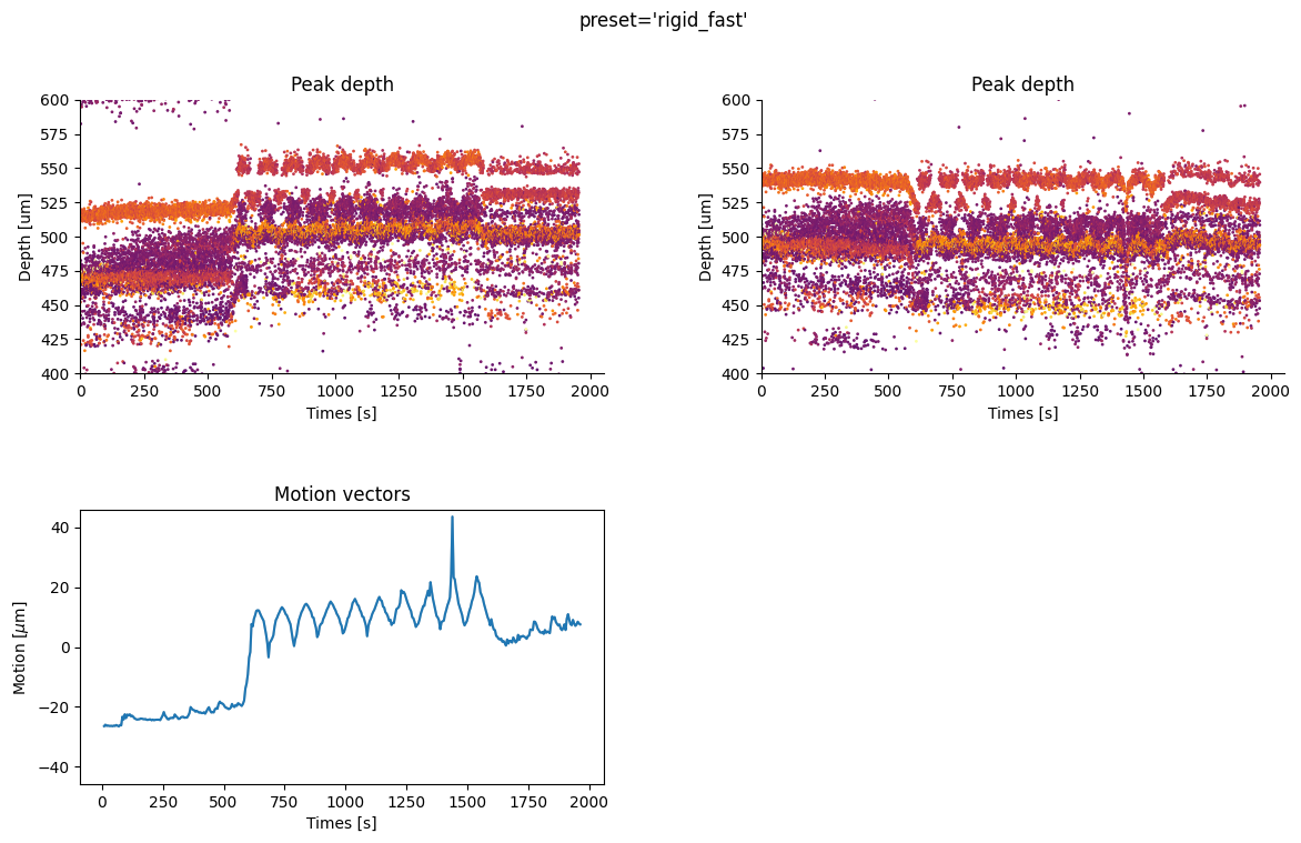
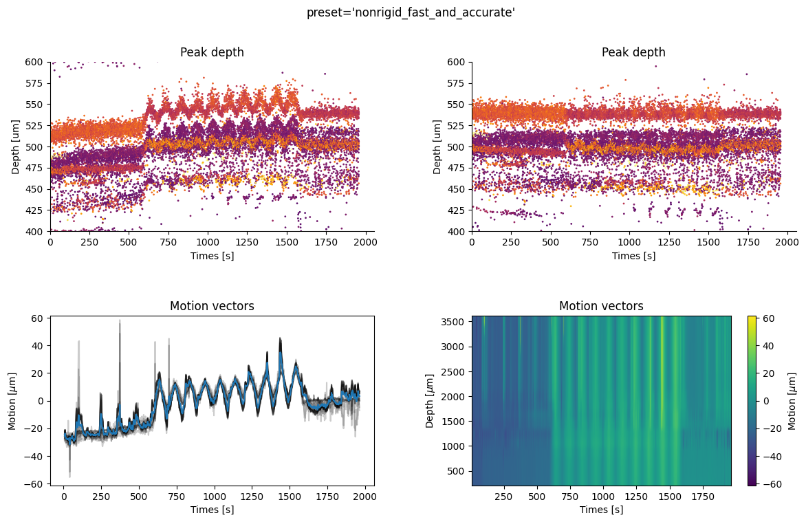
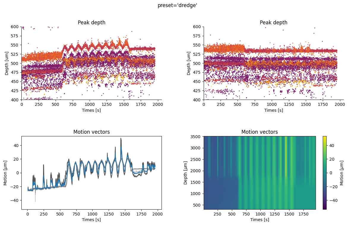
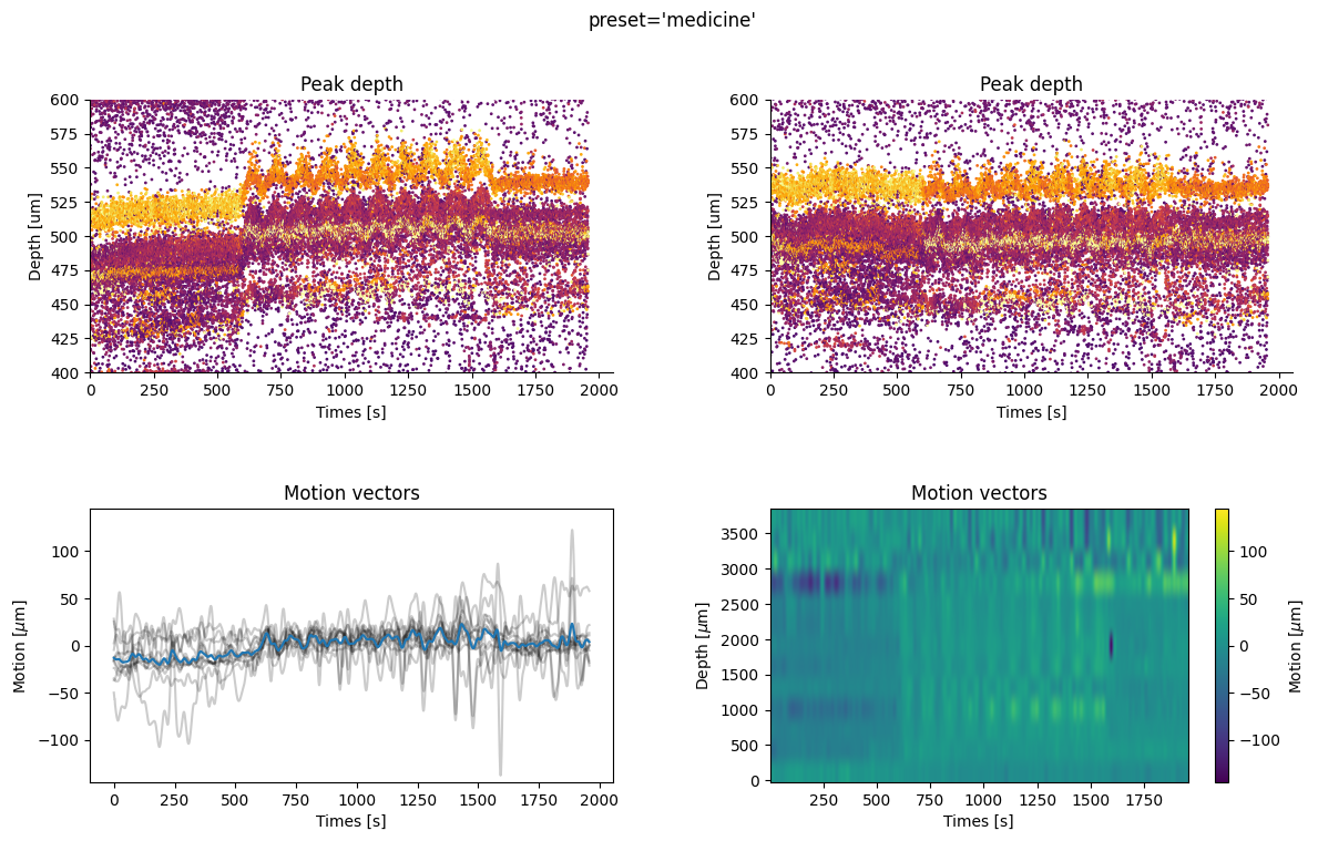
Plot the results
We load back the results and use the widgets module to explore the estimated drift motion.
- For all methods we have 4 plots:
top left: time vs estimated peak
top right: time vs peak depth after motion correction
bottom left: the average motion vector across depths and all motion across spatial depths (for non-rigid estimation)
bottom right: if motion correction is non rigid, the motion vector across depths is plotted as a map, with the color code representing the motion in micrometers.
- A few comments on the figures:
the preset ‘rigid_fast’ has only one motion vector for the entire probe because it is a “rigid” case. The motion amplitude is globally underestimated because it averages across depths. However, the corrected peaks are flatter than the non-corrected ones, so the job is partially done. The big jump at=600s when the probe start moving is recovered quite well.
The preset kilosort_like gives better results because it is a non-rigid case. The motion vector is computed for different depths. The corrected peak locations are flatter than the rigid case. The motion vector map is still be a bit noisy at some depths (e.g around 1000um).
The preset dredge is official DREDge re-implementation in spikeinterface. It give the best result : very fast and smooth motion estimation. Very few noise. This method also capture very well the non rigid motion gradient along the probe. The best method on the market at the moement. An enormous thanks to the dream team : Charlie Windolf, Julien Boussard, Erdem Varol, Liam Paninski. Note that in the first part of the recording before the imposed motion (0-600s) we clearly have a non-rigid motion: the upper part of the probe (2000-3000um) experience some drifts, but the lower part (0-1000um) is relatively stable. The method defined by this preset is able to capture this.
The preset nonrigid_accurate this is the ancestor of “dredge” before it was published. It seems to give good results on this recording but with bit more noise.
The preset dredge_fast similar than dredge but faster (using grid_convolution).
The preset nonrigid_fast_and_accurate a variant of nonrigid_accurate but faster (using grid_convolution).
for preset in some_presets:
    # load
    folder = base_folder / "motion_folder_dataset1" / preset
    motion_info = si.load_motion_info(folder)

    # and plot
    fig = plt.figure(figsize=(14, 8))
    si.plot_motion_info(
        motion_info, rec,
        figure=fig,
        depth_lim=(400, 600),
        color_amplitude=True,
        amplitude_cmap="inferno",
        scatter_decimate=10,
    )

    fig.suptitle(f"{preset=}")


Make an interpolated recording
Once you have analyzed your results you can choose the motion correction
method that works best on your dataset, and create an interpolated
recording using interpolate_motion. The motion object itself is
contained in the motion_info dict. Suppose we decide to use the
nonrigid_accurate preset to make the interpolated recording. We do
this as follows
from spikeinterface.sortingcomponents.motion import interpolate_motion
preset = "nonrigid_accurate"
folder = base_folder / "motion_folder_dataset1" / preset
motion_info = si.load_motion_info(folder)
motion = motion_info['motion']
interpolated_recording = interpolate_motion(recording=rec, motion=motion)
interpolated_recording
Channel IDs
- ['imec0.ap#AP4' 'imec0.ap#AP5' 'imec0.ap#AP6' 'imec0.ap#AP7'
'imec0.ap#AP8' 'imec0.ap#AP9' 'imec0.ap#AP10' 'imec0.ap#AP11'
'imec0.ap#AP12' 'imec0.ap#AP13' 'imec0.ap#AP14' 'imec0.ap#AP15'
'imec0.ap#AP16' 'imec0.ap#AP17' 'imec0.ap#AP18' 'imec0.ap#AP19'
'imec0.ap#AP20' 'imec0.ap#AP21' 'imec0.ap#AP22' 'imec0.ap#AP23'
'imec0.ap#AP24' 'imec0.ap#AP25' 'imec0.ap#AP26' 'imec0.ap#AP27'
'imec0.ap#AP28' 'imec0.ap#AP29' 'imec0.ap#AP30' 'imec0.ap#AP31'
'imec0.ap#AP32' 'imec0.ap#AP33' 'imec0.ap#AP34' 'imec0.ap#AP35'
'imec0.ap#AP36' 'imec0.ap#AP37' 'imec0.ap#AP38' 'imec0.ap#AP39'
'imec0.ap#AP40' 'imec0.ap#AP41' 'imec0.ap#AP42' 'imec0.ap#AP43'
'imec0.ap#AP44' 'imec0.ap#AP45' 'imec0.ap#AP46' 'imec0.ap#AP47'
'imec0.ap#AP48' 'imec0.ap#AP49' 'imec0.ap#AP50' 'imec0.ap#AP51'
'imec0.ap#AP52' 'imec0.ap#AP53' 'imec0.ap#AP54' 'imec0.ap#AP55'
'imec0.ap#AP56' 'imec0.ap#AP57' 'imec0.ap#AP58' 'imec0.ap#AP59'
'imec0.ap#AP60' 'imec0.ap#AP61' 'imec0.ap#AP62' 'imec0.ap#AP63'
'imec0.ap#AP64' 'imec0.ap#AP65' 'imec0.ap#AP66' 'imec0.ap#AP67'
'imec0.ap#AP68' 'imec0.ap#AP69' 'imec0.ap#AP70' 'imec0.ap#AP71'
'imec0.ap#AP72' 'imec0.ap#AP73' 'imec0.ap#AP74' 'imec0.ap#AP75'
'imec0.ap#AP76' 'imec0.ap#AP77' 'imec0.ap#AP78' 'imec0.ap#AP79'
'imec0.ap#AP80' 'imec0.ap#AP81' 'imec0.ap#AP82' 'imec0.ap#AP83'
'imec0.ap#AP84' 'imec0.ap#AP85' 'imec0.ap#AP86' 'imec0.ap#AP87'
'imec0.ap#AP88' 'imec0.ap#AP89' 'imec0.ap#AP90' 'imec0.ap#AP91'
'imec0.ap#AP92' 'imec0.ap#AP93' 'imec0.ap#AP94' 'imec0.ap#AP95'
'imec0.ap#AP96' 'imec0.ap#AP97' 'imec0.ap#AP98' 'imec0.ap#AP99'
'imec0.ap#AP100' 'imec0.ap#AP101' 'imec0.ap#AP102' 'imec0.ap#AP103'
'imec0.ap#AP104' 'imec0.ap#AP105' 'imec0.ap#AP106' 'imec0.ap#AP107'
'imec0.ap#AP108' 'imec0.ap#AP109' 'imec0.ap#AP110' 'imec0.ap#AP111'
'imec0.ap#AP112' 'imec0.ap#AP113' 'imec0.ap#AP114' 'imec0.ap#AP115'
'imec0.ap#AP116' 'imec0.ap#AP117' 'imec0.ap#AP118' 'imec0.ap#AP119'
'imec0.ap#AP120' 'imec0.ap#AP121' 'imec0.ap#AP122' 'imec0.ap#AP123'
'imec0.ap#AP124' 'imec0.ap#AP125' 'imec0.ap#AP126' 'imec0.ap#AP127'
'imec0.ap#AP128' 'imec0.ap#AP129' 'imec0.ap#AP130' 'imec0.ap#AP131'
'imec0.ap#AP132' 'imec0.ap#AP133' 'imec0.ap#AP134' 'imec0.ap#AP135'
'imec0.ap#AP136' 'imec0.ap#AP137' 'imec0.ap#AP138' 'imec0.ap#AP139'
'imec0.ap#AP140' 'imec0.ap#AP141' 'imec0.ap#AP142' 'imec0.ap#AP143'
'imec0.ap#AP144' 'imec0.ap#AP145' 'imec0.ap#AP146' 'imec0.ap#AP147'
'imec0.ap#AP148' 'imec0.ap#AP149' 'imec0.ap#AP150' 'imec0.ap#AP151'
'imec0.ap#AP152' 'imec0.ap#AP153' 'imec0.ap#AP154' 'imec0.ap#AP155'
'imec0.ap#AP156' 'imec0.ap#AP157' 'imec0.ap#AP158' 'imec0.ap#AP159'
'imec0.ap#AP160' 'imec0.ap#AP161' 'imec0.ap#AP162' 'imec0.ap#AP163'
'imec0.ap#AP164' 'imec0.ap#AP165' 'imec0.ap#AP166' 'imec0.ap#AP167'
'imec0.ap#AP168' 'imec0.ap#AP169' 'imec0.ap#AP170' 'imec0.ap#AP171'
'imec0.ap#AP172' 'imec0.ap#AP173' 'imec0.ap#AP174' 'imec0.ap#AP175'
'imec0.ap#AP176' 'imec0.ap#AP177' 'imec0.ap#AP178' 'imec0.ap#AP179'
'imec0.ap#AP180' 'imec0.ap#AP181' 'imec0.ap#AP182' 'imec0.ap#AP183'
'imec0.ap#AP184' 'imec0.ap#AP185' 'imec0.ap#AP186' 'imec0.ap#AP187'
'imec0.ap#AP188' 'imec0.ap#AP189' 'imec0.ap#AP190' 'imec0.ap#AP191'
'imec0.ap#AP192' 'imec0.ap#AP193' 'imec0.ap#AP194' 'imec0.ap#AP195'
'imec0.ap#AP196' 'imec0.ap#AP197' 'imec0.ap#AP198' 'imec0.ap#AP199'
'imec0.ap#AP200' 'imec0.ap#AP201' 'imec0.ap#AP202' 'imec0.ap#AP203'
'imec0.ap#AP204' 'imec0.ap#AP205' 'imec0.ap#AP206' 'imec0.ap#AP207'
'imec0.ap#AP208' 'imec0.ap#AP209' 'imec0.ap#AP210' 'imec0.ap#AP211'
'imec0.ap#AP212' 'imec0.ap#AP213' 'imec0.ap#AP214' 'imec0.ap#AP215'
'imec0.ap#AP216' 'imec0.ap#AP217' 'imec0.ap#AP218' 'imec0.ap#AP219'
'imec0.ap#AP220' 'imec0.ap#AP221' 'imec0.ap#AP222' 'imec0.ap#AP223'
'imec0.ap#AP224' 'imec0.ap#AP225' 'imec0.ap#AP226' 'imec0.ap#AP227'
'imec0.ap#AP228' 'imec0.ap#AP229' 'imec0.ap#AP230' 'imec0.ap#AP231'
'imec0.ap#AP232' 'imec0.ap#AP233' 'imec0.ap#AP234' 'imec0.ap#AP235'
'imec0.ap#AP236' 'imec0.ap#AP237' 'imec0.ap#AP238' 'imec0.ap#AP239'
'imec0.ap#AP240' 'imec0.ap#AP241' 'imec0.ap#AP242' 'imec0.ap#AP243'
'imec0.ap#AP244' 'imec0.ap#AP245' 'imec0.ap#AP246' 'imec0.ap#AP247'
'imec0.ap#AP248' 'imec0.ap#AP249' 'imec0.ap#AP250' 'imec0.ap#AP251'
'imec0.ap#AP252' 'imec0.ap#AP253' 'imec0.ap#AP254' 'imec0.ap#AP255'
'imec0.ap#AP256' 'imec0.ap#AP257' 'imec0.ap#AP258' 'imec0.ap#AP259'
'imec0.ap#AP260' 'imec0.ap#AP261' 'imec0.ap#AP262' 'imec0.ap#AP263'
'imec0.ap#AP264' 'imec0.ap#AP265' 'imec0.ap#AP266' 'imec0.ap#AP267'
'imec0.ap#AP268' 'imec0.ap#AP269' 'imec0.ap#AP270' 'imec0.ap#AP271'
'imec0.ap#AP272' 'imec0.ap#AP273' 'imec0.ap#AP274' 'imec0.ap#AP275'
'imec0.ap#AP276' 'imec0.ap#AP277' 'imec0.ap#AP278' 'imec0.ap#AP279'
'imec0.ap#AP280' 'imec0.ap#AP281' 'imec0.ap#AP282' 'imec0.ap#AP283'
'imec0.ap#AP284' 'imec0.ap#AP285' 'imec0.ap#AP286' 'imec0.ap#AP287'
'imec0.ap#AP288' 'imec0.ap#AP289' 'imec0.ap#AP290' 'imec0.ap#AP291'
'imec0.ap#AP292' 'imec0.ap#AP293' 'imec0.ap#AP294' 'imec0.ap#AP295'
'imec0.ap#AP296' 'imec0.ap#AP297' 'imec0.ap#AP298' 'imec0.ap#AP299'
'imec0.ap#AP300' 'imec0.ap#AP301' 'imec0.ap#AP302' 'imec0.ap#AP303'
'imec0.ap#AP304' 'imec0.ap#AP305' 'imec0.ap#AP306' 'imec0.ap#AP307'
'imec0.ap#AP308' 'imec0.ap#AP309' 'imec0.ap#AP310' 'imec0.ap#AP311'
'imec0.ap#AP312' 'imec0.ap#AP313' 'imec0.ap#AP314' 'imec0.ap#AP315'
'imec0.ap#AP316' 'imec0.ap#AP317' 'imec0.ap#AP318' 'imec0.ap#AP319'
'imec0.ap#AP320' 'imec0.ap#AP321' 'imec0.ap#AP322' 'imec0.ap#AP323'
'imec0.ap#AP324' 'imec0.ap#AP325' 'imec0.ap#AP326' 'imec0.ap#AP327'
'imec0.ap#AP328' 'imec0.ap#AP329' 'imec0.ap#AP330' 'imec0.ap#AP331'
'imec0.ap#AP332' 'imec0.ap#AP333' 'imec0.ap#AP334' 'imec0.ap#AP335'
'imec0.ap#AP336' 'imec0.ap#AP337' 'imec0.ap#AP338' 'imec0.ap#AP339'
'imec0.ap#AP340' 'imec0.ap#AP341' 'imec0.ap#AP342' 'imec0.ap#AP343'
'imec0.ap#AP344' 'imec0.ap#AP345' 'imec0.ap#AP346' 'imec0.ap#AP347'
'imec0.ap#AP348' 'imec0.ap#AP349' 'imec0.ap#AP350' 'imec0.ap#AP351'
'imec0.ap#AP352' 'imec0.ap#AP353' 'imec0.ap#AP354' 'imec0.ap#AP355'
'imec0.ap#AP356' 'imec0.ap#AP357' 'imec0.ap#AP358' 'imec0.ap#AP359'
'imec0.ap#AP360' 'imec0.ap#AP361' 'imec0.ap#AP362' 'imec0.ap#AP363'
'imec0.ap#AP364' 'imec0.ap#AP365' 'imec0.ap#AP366' 'imec0.ap#AP367'
'imec0.ap#AP368' 'imec0.ap#AP369' 'imec0.ap#AP370' 'imec0.ap#AP371'
'imec0.ap#AP372' 'imec0.ap#AP373' 'imec0.ap#AP374' 'imec0.ap#AP375'
'imec0.ap#AP376' 'imec0.ap#AP377']
Annotations
- is_filtered : True
- probe_0_planar_contour : [[ -11 9989] [ -11 -11] [ 24 -186] [ 59 -11] [ 59 9989]]
- probes_info : [{'model_name': 'Neuropixels 1.0', 'manufacturer': 'IMEC', 'shank_tips': [[24, -186]], 'probe_type': '0', 'serial_number': '18408406612', 'part_number': 'PRB_1_4_0480_1_C', 'port': '1', 'slot': '2'}]
Properties
gain_to_uV
[2.34375 2.34375 2.34375 2.34375 2.34375 2.34375 2.34375 2.34375 2.34375 2.34375 2.34375 2.34375 2.34375 2.34375 2.34375 2.34375 2.34375 2.34375 2.34375 2.34375 2.34375 2.34375 2.34375 2.34375 2.34375 2.34375 2.34375 2.34375 2.34375 2.34375 2.34375 2.34375 2.34375 2.34375 2.34375 2.34375 2.34375 2.34375 2.34375 2.34375 2.34375 2.34375 2.34375 2.34375 2.34375 2.34375 2.34375 2.34375 2.34375 2.34375 2.34375 2.34375 2.34375 2.34375 2.34375 2.34375 2.34375 2.34375 2.34375 2.34375 2.34375 2.34375 2.34375 2.34375 2.34375 2.34375 2.34375 2.34375 2.34375 2.34375 2.34375 2.34375 2.34375 2.34375 2.34375 2.34375 2.34375 2.34375 2.34375 2.34375 2.34375 2.34375 2.34375 2.34375 2.34375 2.34375 2.34375 2.34375 2.34375 2.34375 2.34375 2.34375 2.34375 2.34375 2.34375 2.34375 2.34375 2.34375 2.34375 2.34375 2.34375 2.34375 2.34375 2.34375 2.34375 2.34375 2.34375 2.34375 2.34375 2.34375 2.34375 2.34375 2.34375 2.34375 2.34375 2.34375 2.34375 2.34375 2.34375 2.34375 2.34375 2.34375 2.34375 2.34375 2.34375 2.34375 2.34375 2.34375 2.34375 2.34375 2.34375 2.34375 2.34375 2.34375 2.34375 2.34375 2.34375 2.34375 2.34375 2.34375 2.34375 2.34375 2.34375 2.34375 2.34375 2.34375 2.34375 2.34375 2.34375 2.34375 2.34375 2.34375 2.34375 2.34375 2.34375 2.34375 2.34375 2.34375 2.34375 2.34375 2.34375 2.34375 2.34375 2.34375 2.34375 2.34375 2.34375 2.34375 2.34375 2.34375 2.34375 2.34375 2.34375 2.34375 2.34375 2.34375 2.34375 2.34375 2.34375 2.34375 2.34375 2.34375 2.34375 2.34375 2.34375 2.34375 2.34375 2.34375 2.34375 2.34375 2.34375 2.34375 2.34375 2.34375 2.34375 2.34375 2.34375 2.34375 2.34375 2.34375 2.34375 2.34375 2.34375 2.34375 2.34375 2.34375 2.34375 2.34375 2.34375 2.34375 2.34375 2.34375 2.34375 2.34375 2.34375 2.34375 2.34375 2.34375 2.34375 2.34375 2.34375 2.34375 2.34375 2.34375 2.34375 2.34375 2.34375 2.34375 2.34375 2.34375 2.34375 2.34375 2.34375 2.34375 2.34375 2.34375 2.34375 2.34375 2.34375 2.34375 2.34375 2.34375 2.34375 2.34375 2.34375 2.34375 2.34375 2.34375 2.34375 2.34375 2.34375 2.34375 2.34375 2.34375 2.34375 2.34375 2.34375 2.34375 2.34375 2.34375 2.34375 2.34375 2.34375 2.34375 2.34375 2.34375 2.34375 2.34375 2.34375 2.34375 2.34375 2.34375 2.34375 2.34375 2.34375 2.34375 2.34375 2.34375 2.34375 2.34375 2.34375 2.34375 2.34375 2.34375 2.34375 2.34375 2.34375 2.34375 2.34375 2.34375 2.34375 2.34375 2.34375 2.34375 2.34375 2.34375 2.34375 2.34375 2.34375 2.34375 2.34375 2.34375 2.34375 2.34375 2.34375 2.34375 2.34375 2.34375 2.34375 2.34375 2.34375 2.34375 2.34375 2.34375 2.34375 2.34375 2.34375 2.34375 2.34375 2.34375 2.34375 2.34375 2.34375 2.34375 2.34375 2.34375 2.34375 2.34375 2.34375 2.34375 2.34375 2.34375 2.34375 2.34375 2.34375 2.34375 2.34375 2.34375 2.34375 2.34375 2.34375 2.34375 2.34375 2.34375 2.34375 2.34375 2.34375 2.34375 2.34375 2.34375 2.34375 2.34375 2.34375 2.34375 2.34375 2.34375 2.34375 2.34375 2.34375 2.34375 2.34375 2.34375 2.34375 2.34375 2.34375 2.34375 2.34375 2.34375 2.34375 2.34375 2.34375 2.34375 2.34375 2.34375]offset_to_uV
[0 0 0 0 0 0 0 0 0 0 0 0 0 0 0 0 0 0 0 0 0 0 0 0 0 0 0 0 0 0 0 0 0 0 0 0 0 0 0 0 0 0 0 0 0 0 0 0 0 0 0 0 0 0 0 0 0 0 0 0 0 0 0 0 0 0 0 0 0 0 0 0 0 0 0 0 0 0 0 0 0 0 0 0 0 0 0 0 0 0 0 0 0 0 0 0 0 0 0 0 0 0 0 0 0 0 0 0 0 0 0 0 0 0 0 0 0 0 0 0 0 0 0 0 0 0 0 0 0 0 0 0 0 0 0 0 0 0 0 0 0 0 0 0 0 0 0 0 0 0 0 0 0 0 0 0 0 0 0 0 0 0 0 0 0 0 0 0 0 0 0 0 0 0 0 0 0 0 0 0 0 0 0 0 0 0 0 0 0 0 0 0 0 0 0 0 0 0 0 0 0 0 0 0 0 0 0 0 0 0 0 0 0 0 0 0 0 0 0 0 0 0 0 0 0 0 0 0 0 0 0 0 0 0 0 0 0 0 0 0 0 0 0 0 0 0 0 0 0 0 0 0 0 0 0 0 0 0 0 0 0 0 0 0 0 0 0 0 0 0 0 0 0 0 0 0 0 0 0 0 0 0 0 0 0 0 0 0 0 0 0 0 0 0 0 0 0 0 0 0 0 0 0 0 0 0 0 0 0 0 0 0 0 0 0 0 0 0 0 0 0 0 0 0 0 0 0 0 0 0 0 0 0 0 0 0 0 0 0 0 0 0 0 0 0 0 0 0 0 0 0 0 0 0 0 0 0 0 0 0 0 0 0 0 0 0 0 0 0 0 0 0 0 0]physical_unit
['uV' 'uV' 'uV' 'uV' 'uV' 'uV' 'uV' 'uV' 'uV' 'uV' 'uV' 'uV' 'uV' 'uV' 'uV' 'uV' 'uV' 'uV' 'uV' 'uV' 'uV' 'uV' 'uV' 'uV' 'uV' 'uV' 'uV' 'uV' 'uV' 'uV' 'uV' 'uV' 'uV' 'uV' 'uV' 'uV' 'uV' 'uV' 'uV' 'uV' 'uV' 'uV' 'uV' 'uV' 'uV' 'uV' 'uV' 'uV' 'uV' 'uV' 'uV' 'uV' 'uV' 'uV' 'uV' 'uV' 'uV' 'uV' 'uV' 'uV' 'uV' 'uV' 'uV' 'uV' 'uV' 'uV' 'uV' 'uV' 'uV' 'uV' 'uV' 'uV' 'uV' 'uV' 'uV' 'uV' 'uV' 'uV' 'uV' 'uV' 'uV' 'uV' 'uV' 'uV' 'uV' 'uV' 'uV' 'uV' 'uV' 'uV' 'uV' 'uV' 'uV' 'uV' 'uV' 'uV' 'uV' 'uV' 'uV' 'uV' 'uV' 'uV' 'uV' 'uV' 'uV' 'uV' 'uV' 'uV' 'uV' 'uV' 'uV' 'uV' 'uV' 'uV' 'uV' 'uV' 'uV' 'uV' 'uV' 'uV' 'uV' 'uV' 'uV' 'uV' 'uV' 'uV' 'uV' 'uV' 'uV' 'uV' 'uV' 'uV' 'uV' 'uV' 'uV' 'uV' 'uV' 'uV' 'uV' 'uV' 'uV' 'uV' 'uV' 'uV' 'uV' 'uV' 'uV' 'uV' 'uV' 'uV' 'uV' 'uV' 'uV' 'uV' 'uV' 'uV' 'uV' 'uV' 'uV' 'uV' 'uV' 'uV' 'uV' 'uV' 'uV' 'uV' 'uV' 'uV' 'uV' 'uV' 'uV' 'uV' 'uV' 'uV' 'uV' 'uV' 'uV' 'uV' 'uV' 'uV' 'uV' 'uV' 'uV' 'uV' 'uV' 'uV' 'uV' 'uV' 'uV' 'uV' 'uV' 'uV' 'uV' 'uV' 'uV' 'uV' 'uV' 'uV' 'uV' 'uV' 'uV' 'uV' 'uV' 'uV' 'uV' 'uV' 'uV' 'uV' 'uV' 'uV' 'uV' 'uV' 'uV' 'uV' 'uV' 'uV' 'uV' 'uV' 'uV' 'uV' 'uV' 'uV' 'uV' 'uV' 'uV' 'uV' 'uV' 'uV' 'uV' 'uV' 'uV' 'uV' 'uV' 'uV' 'uV' 'uV' 'uV' 'uV' 'uV' 'uV' 'uV' 'uV' 'uV' 'uV' 'uV' 'uV' 'uV' 'uV' 'uV' 'uV' 'uV' 'uV' 'uV' 'uV' 'uV' 'uV' 'uV' 'uV' 'uV' 'uV' 'uV' 'uV' 'uV' 'uV' 'uV' 'uV' 'uV' 'uV' 'uV' 'uV' 'uV' 'uV' 'uV' 'uV' 'uV' 'uV' 'uV' 'uV' 'uV' 'uV' 'uV' 'uV' 'uV' 'uV' 'uV' 'uV' 'uV' 'uV' 'uV' 'uV' 'uV' 'uV' 'uV' 'uV' 'uV' 'uV' 'uV' 'uV' 'uV' 'uV' 'uV' 'uV' 'uV' 'uV' 'uV' 'uV' 'uV' 'uV' 'uV' 'uV' 'uV' 'uV' 'uV' 'uV' 'uV' 'uV' 'uV' 'uV' 'uV' 'uV' 'uV' 'uV' 'uV' 'uV' 'uV' 'uV' 'uV' 'uV' 'uV' 'uV' 'uV' 'uV' 'uV' 'uV' 'uV' 'uV' 'uV' 'uV' 'uV' 'uV' 'uV' 'uV' 'uV' 'uV' 'uV' 'uV' 'uV' 'uV' 'uV' 'uV' 'uV' 'uV' 'uV' 'uV' 'uV' 'uV' 'uV' 'uV' 'uV' 'uV' 'uV' 'uV' 'uV' 'uV' 'uV' 'uV' 'uV' 'uV' 'uV' 'uV' 'uV' 'uV' 'uV' 'uV']gain_to_physical_unit
[2.34375 2.34375 2.34375 2.34375 2.34375 2.34375 2.34375 2.34375 2.34375 2.34375 2.34375 2.34375 2.34375 2.34375 2.34375 2.34375 2.34375 2.34375 2.34375 2.34375 2.34375 2.34375 2.34375 2.34375 2.34375 2.34375 2.34375 2.34375 2.34375 2.34375 2.34375 2.34375 2.34375 2.34375 2.34375 2.34375 2.34375 2.34375 2.34375 2.34375 2.34375 2.34375 2.34375 2.34375 2.34375 2.34375 2.34375 2.34375 2.34375 2.34375 2.34375 2.34375 2.34375 2.34375 2.34375 2.34375 2.34375 2.34375 2.34375 2.34375 2.34375 2.34375 2.34375 2.34375 2.34375 2.34375 2.34375 2.34375 2.34375 2.34375 2.34375 2.34375 2.34375 2.34375 2.34375 2.34375 2.34375 2.34375 2.34375 2.34375 2.34375 2.34375 2.34375 2.34375 2.34375 2.34375 2.34375 2.34375 2.34375 2.34375 2.34375 2.34375 2.34375 2.34375 2.34375 2.34375 2.34375 2.34375 2.34375 2.34375 2.34375 2.34375 2.34375 2.34375 2.34375 2.34375 2.34375 2.34375 2.34375 2.34375 2.34375 2.34375 2.34375 2.34375 2.34375 2.34375 2.34375 2.34375 2.34375 2.34375 2.34375 2.34375 2.34375 2.34375 2.34375 2.34375 2.34375 2.34375 2.34375 2.34375 2.34375 2.34375 2.34375 2.34375 2.34375 2.34375 2.34375 2.34375 2.34375 2.34375 2.34375 2.34375 2.34375 2.34375 2.34375 2.34375 2.34375 2.34375 2.34375 2.34375 2.34375 2.34375 2.34375 2.34375 2.34375 2.34375 2.34375 2.34375 2.34375 2.34375 2.34375 2.34375 2.34375 2.34375 2.34375 2.34375 2.34375 2.34375 2.34375 2.34375 2.34375 2.34375 2.34375 2.34375 2.34375 2.34375 2.34375 2.34375 2.34375 2.34375 2.34375 2.34375 2.34375 2.34375 2.34375 2.34375 2.34375 2.34375 2.34375 2.34375 2.34375 2.34375 2.34375 2.34375 2.34375 2.34375 2.34375 2.34375 2.34375 2.34375 2.34375 2.34375 2.34375 2.34375 2.34375 2.34375 2.34375 2.34375 2.34375 2.34375 2.34375 2.34375 2.34375 2.34375 2.34375 2.34375 2.34375 2.34375 2.34375 2.34375 2.34375 2.34375 2.34375 2.34375 2.34375 2.34375 2.34375 2.34375 2.34375 2.34375 2.34375 2.34375 2.34375 2.34375 2.34375 2.34375 2.34375 2.34375 2.34375 2.34375 2.34375 2.34375 2.34375 2.34375 2.34375 2.34375 2.34375 2.34375 2.34375 2.34375 2.34375 2.34375 2.34375 2.34375 2.34375 2.34375 2.34375 2.34375 2.34375 2.34375 2.34375 2.34375 2.34375 2.34375 2.34375 2.34375 2.34375 2.34375 2.34375 2.34375 2.34375 2.34375 2.34375 2.34375 2.34375 2.34375 2.34375 2.34375 2.34375 2.34375 2.34375 2.34375 2.34375 2.34375 2.34375 2.34375 2.34375 2.34375 2.34375 2.34375 2.34375 2.34375 2.34375 2.34375 2.34375 2.34375 2.34375 2.34375 2.34375 2.34375 2.34375 2.34375 2.34375 2.34375 2.34375 2.34375 2.34375 2.34375 2.34375 2.34375 2.34375 2.34375 2.34375 2.34375 2.34375 2.34375 2.34375 2.34375 2.34375 2.34375 2.34375 2.34375 2.34375 2.34375 2.34375 2.34375 2.34375 2.34375 2.34375 2.34375 2.34375 2.34375 2.34375 2.34375 2.34375 2.34375 2.34375 2.34375 2.34375 2.34375 2.34375 2.34375 2.34375 2.34375 2.34375 2.34375 2.34375 2.34375 2.34375 2.34375 2.34375 2.34375 2.34375 2.34375 2.34375 2.34375 2.34375 2.34375 2.34375 2.34375 2.34375 2.34375 2.34375 2.34375 2.34375 2.34375 2.34375 2.34375 2.34375 2.34375 2.34375 2.34375 2.34375 2.34375]offset_to_physical_unit
[0. 0. 0. 0. 0. 0. 0. 0. 0. 0. 0. 0. 0. 0. 0. 0. 0. 0. 0. 0. 0. 0. 0. 0. 0. 0. 0. 0. 0. 0. 0. 0. 0. 0. 0. 0. 0. 0. 0. 0. 0. 0. 0. 0. 0. 0. 0. 0. 0. 0. 0. 0. 0. 0. 0. 0. 0. 0. 0. 0. 0. 0. 0. 0. 0. 0. 0. 0. 0. 0. 0. 0. 0. 0. 0. 0. 0. 0. 0. 0. 0. 0. 0. 0. 0. 0. 0. 0. 0. 0. 0. 0. 0. 0. 0. 0. 0. 0. 0. 0. 0. 0. 0. 0. 0. 0. 0. 0. 0. 0. 0. 0. 0. 0. 0. 0. 0. 0. 0. 0. 0. 0. 0. 0. 0. 0. 0. 0. 0. 0. 0. 0. 0. 0. 0. 0. 0. 0. 0. 0. 0. 0. 0. 0. 0. 0. 0. 0. 0. 0. 0. 0. 0. 0. 0. 0. 0. 0. 0. 0. 0. 0. 0. 0. 0. 0. 0. 0. 0. 0. 0. 0. 0. 0. 0. 0. 0. 0. 0. 0. 0. 0. 0. 0. 0. 0. 0. 0. 0. 0. 0. 0. 0. 0. 0. 0. 0. 0. 0. 0. 0. 0. 0. 0. 0. 0. 0. 0. 0. 0. 0. 0. 0. 0. 0. 0. 0. 0. 0. 0. 0. 0. 0. 0. 0. 0. 0. 0. 0. 0. 0. 0. 0. 0. 0. 0. 0. 0. 0. 0. 0. 0. 0. 0. 0. 0. 0. 0. 0. 0. 0. 0. 0. 0. 0. 0. 0. 0. 0. 0. 0. 0. 0. 0. 0. 0. 0. 0. 0. 0. 0. 0. 0. 0. 0. 0. 0. 0. 0. 0. 0. 0. 0. 0. 0. 0. 0. 0. 0. 0. 0. 0. 0. 0. 0. 0. 0. 0. 0. 0. 0. 0. 0. 0. 0. 0. 0. 0. 0. 0. 0. 0. 0. 0. 0. 0. 0. 0. 0. 0. 0. 0. 0. 0. 0. 0. 0. 0. 0. 0. 0. 0. 0. 0. 0. 0. 0. 0. 0. 0. 0. 0. 0. 0. 0. 0. 0. 0. 0. 0. 0. 0. 0. 0. 0. 0. 0. 0. 0. 0. 0. 0. 0. 0. 0. 0. 0. 0. 0. 0. 0. 0. 0. 0.]channel_name
['AP4' 'AP5' 'AP6' 'AP7' 'AP8' 'AP9' 'AP10' 'AP11' 'AP12' 'AP13' 'AP14' 'AP15' 'AP16' 'AP17' 'AP18' 'AP19' 'AP20' 'AP21' 'AP22' 'AP23' 'AP24' 'AP25' 'AP26' 'AP27' 'AP28' 'AP29' 'AP30' 'AP31' 'AP32' 'AP33' 'AP34' 'AP35' 'AP36' 'AP37' 'AP38' 'AP39' 'AP40' 'AP41' 'AP42' 'AP43' 'AP44' 'AP45' 'AP46' 'AP47' 'AP48' 'AP49' 'AP50' 'AP51' 'AP52' 'AP53' 'AP54' 'AP55' 'AP56' 'AP57' 'AP58' 'AP59' 'AP60' 'AP61' 'AP62' 'AP63' 'AP64' 'AP65' 'AP66' 'AP67' 'AP68' 'AP69' 'AP70' 'AP71' 'AP72' 'AP73' 'AP74' 'AP75' 'AP76' 'AP77' 'AP78' 'AP79' 'AP80' 'AP81' 'AP82' 'AP83' 'AP84' 'AP85' 'AP86' 'AP87' 'AP88' 'AP89' 'AP90' 'AP91' 'AP92' 'AP93' 'AP94' 'AP95' 'AP96' 'AP97' 'AP98' 'AP99' 'AP100' 'AP101' 'AP102' 'AP103' 'AP104' 'AP105' 'AP106' 'AP107' 'AP108' 'AP109' 'AP110' 'AP111' 'AP112' 'AP113' 'AP114' 'AP115' 'AP116' 'AP117' 'AP118' 'AP119' 'AP120' 'AP121' 'AP122' 'AP123' 'AP124' 'AP125' 'AP126' 'AP127' 'AP128' 'AP129' 'AP130' 'AP131' 'AP132' 'AP133' 'AP134' 'AP135' 'AP136' 'AP137' 'AP138' 'AP139' 'AP140' 'AP141' 'AP142' 'AP143' 'AP144' 'AP145' 'AP146' 'AP147' 'AP148' 'AP149' 'AP150' 'AP151' 'AP152' 'AP153' 'AP154' 'AP155' 'AP156' 'AP157' 'AP158' 'AP159' 'AP160' 'AP161' 'AP162' 'AP163' 'AP164' 'AP165' 'AP166' 'AP167' 'AP168' 'AP169' 'AP170' 'AP171' 'AP172' 'AP173' 'AP174' 'AP175' 'AP176' 'AP177' 'AP178' 'AP179' 'AP180' 'AP181' 'AP182' 'AP183' 'AP184' 'AP185' 'AP186' 'AP187' 'AP188' 'AP189' 'AP190' 'AP191' 'AP192' 'AP193' 'AP194' 'AP195' 'AP196' 'AP197' 'AP198' 'AP199' 'AP200' 'AP201' 'AP202' 'AP203' 'AP204' 'AP205' 'AP206' 'AP207' 'AP208' 'AP209' 'AP210' 'AP211' 'AP212' 'AP213' 'AP214' 'AP215' 'AP216' 'AP217' 'AP218' 'AP219' 'AP220' 'AP221' 'AP222' 'AP223' 'AP224' 'AP225' 'AP226' 'AP227' 'AP228' 'AP229' 'AP230' 'AP231' 'AP232' 'AP233' 'AP234' 'AP235' 'AP236' 'AP237' 'AP238' 'AP239' 'AP240' 'AP241' 'AP242' 'AP243' 'AP244' 'AP245' 'AP246' 'AP247' 'AP248' 'AP249' 'AP250' 'AP251' 'AP252' 'AP253' 'AP254' 'AP255' 'AP256' 'AP257' 'AP258' 'AP259' 'AP260' 'AP261' 'AP262' 'AP263' 'AP264' 'AP265' 'AP266' 'AP267' 'AP268' 'AP269' 'AP270' 'AP271' 'AP272' 'AP273' 'AP274' 'AP275' 'AP276' 'AP277' 'AP278' 'AP279' 'AP280' 'AP281' 'AP282' 'AP283' 'AP284' 'AP285' 'AP286' 'AP287' 'AP288' 'AP289' 'AP290' 'AP291' 'AP292' 'AP293' 'AP294' 'AP295' 'AP296' 'AP297' 'AP298' 'AP299' 'AP300' 'AP301' 'AP302' 'AP303' 'AP304' 'AP305' 'AP306' 'AP307' 'AP308' 'AP309' 'AP310' 'AP311' 'AP312' 'AP313' 'AP314' 'AP315' 'AP316' 'AP317' 'AP318' 'AP319' 'AP320' 'AP321' 'AP322' 'AP323' 'AP324' 'AP325' 'AP326' 'AP327' 'AP328' 'AP329' 'AP330' 'AP331' 'AP332' 'AP333' 'AP334' 'AP335' 'AP336' 'AP337' 'AP338' 'AP339' 'AP340' 'AP341' 'AP342' 'AP343' 'AP344' 'AP345' 'AP346' 'AP347' 'AP348' 'AP349' 'AP350' 'AP351' 'AP352' 'AP353' 'AP354' 'AP355' 'AP356' 'AP357' 'AP358' 'AP359' 'AP360' 'AP361' 'AP362' 'AP363' 'AP364' 'AP365' 'AP366' 'AP367' 'AP368' 'AP369' 'AP370' 'AP371' 'AP372' 'AP373' 'AP374' 'AP375' 'AP376' 'AP377']contact_vector
[(0, 16., 40., 'square', 12., '', 'e4', 0, 'um', 1., 0., 0., 1., 4, 0, 0, 500, 250, 1) (0, 48., 40., 'square', 12., '', 'e5', 1, 'um', 1., 0., 0., 1., 5, 0, 0, 500, 250, 1) (0, 0., 60., 'square', 12., '', 'e6', 2, 'um', 1., 0., 0., 1., 6, 0, 0, 500, 250, 1) (0, 32., 60., 'square', 12., '', 'e7', 3, 'um', 1., 0., 0., 1., 7, 0, 0, 500, 250, 1) (0, 16., 80., 'square', 12., '', 'e8', 4, 'um', 1., 0., 0., 1., 8, 0, 0, 500, 250, 1) (0, 48., 80., 'square', 12., '', 'e9', 5, 'um', 1., 0., 0., 1., 9, 0, 0, 500, 250, 1) (0, 0., 100., 'square', 12., '', 'e10', 6, 'um', 1., 0., 0., 1., 10, 0, 0, 500, 250, 1) (0, 32., 100., 'square', 12., '', 'e11', 7, 'um', 1., 0., 0., 1., 11, 0, 0, 500, 250, 1) (0, 16., 120., 'square', 12., '', 'e12', 8, 'um', 1., 0., 0., 1., 12, 0, 0, 500, 250, 1) (0, 48., 120., 'square', 12., '', 'e13', 9, 'um', 1., 0., 0., 1., 13, 0, 0, 500, 250, 1) (0, 0., 140., 'square', 12., '', 'e14', 10, 'um', 1., 0., 0., 1., 14, 0, 0, 500, 250, 1) (0, 32., 140., 'square', 12., '', 'e15', 11, 'um', 1., 0., 0., 1., 15, 0, 0, 500, 250, 1) (0, 16., 160., 'square', 12., '', 'e16', 12, 'um', 1., 0., 0., 1., 16, 0, 0, 500, 250, 1) (0, 48., 160., 'square', 12., '', 'e17', 13, 'um', 1., 0., 0., 1., 17, 0, 0, 500, 250, 1) (0, 0., 180., 'square', 12., '', 'e18', 14, 'um', 1., 0., 0., 1., 18, 0, 0, 500, 250, 1) (0, 32., 180., 'square', 12., '', 'e19', 15, 'um', 1., 0., 0., 1., 19, 0, 0, 500, 250, 1) (0, 16., 200., 'square', 12., '', 'e20', 16, 'um', 1., 0., 0., 1., 20, 0, 0, 500, 250, 1) (0, 48., 200., 'square', 12., '', 'e21', 17, 'um', 1., 0., 0., 1., 21, 0, 0, 500, 250, 1) (0, 0., 220., 'square', 12., '', 'e22', 18, 'um', 1., 0., 0., 1., 22, 0, 0, 500, 250, 1) (0, 32., 220., 'square', 12., '', 'e23', 19, 'um', 1., 0., 0., 1., 23, 0, 0, 500, 250, 1) (0, 16., 240., 'square', 12., '', 'e24', 20, 'um', 1., 0., 0., 1., 24, 0, 0, 500, 250, 1) (0, 48., 240., 'square', 12., '', 'e25', 21, 'um', 1., 0., 0., 1., 25, 0, 0, 500, 250, 1) (0, 0., 260., 'square', 12., '', 'e26', 22, 'um', 1., 0., 0., 1., 26, 0, 0, 500, 250, 1) (0, 32., 260., 'square', 12., '', 'e27', 23, 'um', 1., 0., 0., 1., 27, 0, 0, 500, 250, 1) (0, 16., 280., 'square', 12., '', 'e28', 24, 'um', 1., 0., 0., 1., 28, 0, 0, 500, 250, 1) (0, 48., 280., 'square', 12., '', 'e29', 25, 'um', 1., 0., 0., 1., 29, 0, 0, 500, 250, 1) (0, 0., 300., 'square', 12., '', 'e30', 26, 'um', 1., 0., 0., 1., 30, 0, 0, 500, 250, 1) (0, 32., 300., 'square', 12., '', 'e31', 27, 'um', 1., 0., 0., 1., 31, 0, 0, 500, 250, 1) (0, 16., 320., 'square', 12., '', 'e32', 28, 'um', 1., 0., 0., 1., 32, 0, 0, 500, 250, 1) (0, 48., 320., 'square', 12., '', 'e33', 29, 'um', 1., 0., 0., 1., 33, 0, 0, 500, 250, 1) (0, 0., 340., 'square', 12., '', 'e34', 30, 'um', 1., 0., 0., 1., 34, 0, 0, 500, 250, 1) (0, 32., 340., 'square', 12., '', 'e35', 31, 'um', 1., 0., 0., 1., 35, 0, 0, 500, 250, 1) (0, 16., 360., 'square', 12., '', 'e36', 32, 'um', 1., 0., 0., 1., 36, 0, 0, 500, 250, 1) (0, 48., 360., 'square', 12., '', 'e37', 33, 'um', 1., 0., 0., 1., 37, 0, 0, 500, 250, 1) (0, 0., 380., 'square', 12., '', 'e38', 34, 'um', 1., 0., 0., 1., 38, 0, 0, 500, 250, 1) (0, 32., 380., 'square', 12., '', 'e39', 35, 'um', 1., 0., 0., 1., 39, 0, 0, 500, 250, 1) (0, 16., 400., 'square', 12., '', 'e40', 36, 'um', 1., 0., 0., 1., 40, 0, 0, 500, 250, 1) (0, 48., 400., 'square', 12., '', 'e41', 37, 'um', 1., 0., 0., 1., 41, 0, 0, 500, 250, 1) (0, 0., 420., 'square', 12., '', 'e42', 38, 'um', 1., 0., 0., 1., 42, 0, 0, 500, 250, 1) (0, 32., 420., 'square', 12., '', 'e43', 39, 'um', 1., 0., 0., 1., 43, 0, 0, 500, 250, 1) (0, 16., 440., 'square', 12., '', 'e44', 40, 'um', 1., 0., 0., 1., 44, 0, 0, 500, 250, 1) (0, 48., 440., 'square', 12., '', 'e45', 41, 'um', 1., 0., 0., 1., 45, 0, 0, 500, 250, 1) (0, 0., 460., 'square', 12., '', 'e46', 42, 'um', 1., 0., 0., 1., 46, 0, 0, 500, 250, 1) (0, 32., 460., 'square', 12., '', 'e47', 43, 'um', 1., 0., 0., 1., 47, 0, 0, 500, 250, 1) (0, 16., 480., 'square', 12., '', 'e48', 44, 'um', 1., 0., 0., 1., 48, 0, 0, 500, 250, 1) (0, 48., 480., 'square', 12., '', 'e49', 45, 'um', 1., 0., 0., 1., 49, 0, 0, 500, 250, 1) (0, 0., 500., 'square', 12., '', 'e50', 46, 'um', 1., 0., 0., 1., 50, 0, 0, 500, 250, 1) (0, 32., 500., 'square', 12., '', 'e51', 47, 'um', 1., 0., 0., 1., 51, 0, 0, 500, 250, 1) (0, 16., 520., 'square', 12., '', 'e52', 48, 'um', 1., 0., 0., 1., 52, 0, 0, 500, 250, 1) (0, 48., 520., 'square', 12., '', 'e53', 49, 'um', 1., 0., 0., 1., 53, 0, 0, 500, 250, 1) (0, 0., 540., 'square', 12., '', 'e54', 50, 'um', 1., 0., 0., 1., 54, 0, 0, 500, 250, 1) (0, 32., 540., 'square', 12., '', 'e55', 51, 'um', 1., 0., 0., 1., 55, 0, 0, 500, 250, 1) (0, 16., 560., 'square', 12., '', 'e56', 52, 'um', 1., 0., 0., 1., 56, 0, 0, 500, 250, 1) (0, 48., 560., 'square', 12., '', 'e57', 53, 'um', 1., 0., 0., 1., 57, 0, 0, 500, 250, 1) (0, 0., 580., 'square', 12., '', 'e58', 54, 'um', 1., 0., 0., 1., 58, 0, 0, 500, 250, 1) (0, 32., 580., 'square', 12., '', 'e59', 55, 'um', 1., 0., 0., 1., 59, 0, 0, 500, 250, 1) (0, 16., 600., 'square', 12., '', 'e60', 56, 'um', 1., 0., 0., 1., 60, 0, 0, 500, 250, 1) (0, 48., 600., 'square', 12., '', 'e61', 57, 'um', 1., 0., 0., 1., 61, 0, 0, 500, 250, 1) (0, 0., 620., 'square', 12., '', 'e62', 58, 'um', 1., 0., 0., 1., 62, 0, 0, 500, 250, 1) (0, 32., 620., 'square', 12., '', 'e63', 59, 'um', 1., 0., 0., 1., 63, 0, 0, 500, 250, 1) (0, 16., 640., 'square', 12., '', 'e64', 60, 'um', 1., 0., 0., 1., 64, 0, 0, 500, 250, 1) (0, 48., 640., 'square', 12., '', 'e65', 61, 'um', 1., 0., 0., 1., 65, 0, 0, 500, 250, 1) (0, 0., 660., 'square', 12., '', 'e66', 62, 'um', 1., 0., 0., 1., 66, 0, 0, 500, 250, 1) (0, 32., 660., 'square', 12., '', 'e67', 63, 'um', 1., 0., 0., 1., 67, 0, 0, 500, 250, 1) (0, 16., 680., 'square', 12., '', 'e68', 64, 'um', 1., 0., 0., 1., 68, 0, 0, 500, 250, 1) (0, 48., 680., 'square', 12., '', 'e69', 65, 'um', 1., 0., 0., 1., 69, 0, 0, 500, 250, 1) (0, 0., 700., 'square', 12., '', 'e70', 66, 'um', 1., 0., 0., 1., 70, 0, 0, 500, 250, 1) (0, 32., 700., 'square', 12., '', 'e71', 67, 'um', 1., 0., 0., 1., 71, 0, 0, 500, 250, 1) (0, 16., 720., 'square', 12., '', 'e72', 68, 'um', 1., 0., 0., 1., 72, 0, 0, 500, 250, 1) (0, 48., 720., 'square', 12., '', 'e73', 69, 'um', 1., 0., 0., 1., 73, 0, 0, 500, 250, 1) (0, 0., 740., 'square', 12., '', 'e74', 70, 'um', 1., 0., 0., 1., 74, 0, 0, 500, 250, 1) (0, 32., 740., 'square', 12., '', 'e75', 71, 'um', 1., 0., 0., 1., 75, 0, 0, 500, 250, 1) (0, 16., 760., 'square', 12., '', 'e76', 72, 'um', 1., 0., 0., 1., 76, 0, 0, 500, 250, 1) (0, 48., 760., 'square', 12., '', 'e77', 73, 'um', 1., 0., 0., 1., 77, 0, 0, 500, 250, 1) (0, 0., 780., 'square', 12., '', 'e78', 74, 'um', 1., 0., 0., 1., 78, 0, 0, 500, 250, 1) (0, 32., 780., 'square', 12., '', 'e79', 75, 'um', 1., 0., 0., 1., 79, 0, 0, 500, 250, 1) (0, 16., 800., 'square', 12., '', 'e80', 76, 'um', 1., 0., 0., 1., 80, 0, 0, 500, 250, 1) (0, 48., 800., 'square', 12., '', 'e81', 77, 'um', 1., 0., 0., 1., 81, 0, 0, 500, 250, 1) (0, 0., 820., 'square', 12., '', 'e82', 78, 'um', 1., 0., 0., 1., 82, 0, 0, 500, 250, 1) (0, 32., 820., 'square', 12., '', 'e83', 79, 'um', 1., 0., 0., 1., 83, 0, 0, 500, 250, 1) (0, 16., 840., 'square', 12., '', 'e84', 80, 'um', 1., 0., 0., 1., 84, 0, 0, 500, 250, 1) (0, 48., 840., 'square', 12., '', 'e85', 81, 'um', 1., 0., 0., 1., 85, 0, 0, 500, 250, 1) (0, 0., 860., 'square', 12., '', 'e86', 82, 'um', 1., 0., 0., 1., 86, 0, 0, 500, 250, 1) (0, 32., 860., 'square', 12., '', 'e87', 83, 'um', 1., 0., 0., 1., 87, 0, 0, 500, 250, 1) (0, 16., 880., 'square', 12., '', 'e88', 84, 'um', 1., 0., 0., 1., 88, 0, 0, 500, 250, 1) (0, 48., 880., 'square', 12., '', 'e89', 85, 'um', 1., 0., 0., 1., 89, 0, 0, 500, 250, 1) (0, 0., 900., 'square', 12., '', 'e90', 86, 'um', 1., 0., 0., 1., 90, 0, 0, 500, 250, 1) (0, 32., 900., 'square', 12., '', 'e91', 87, 'um', 1., 0., 0., 1., 91, 0, 0, 500, 250, 1) (0, 16., 920., 'square', 12., '', 'e92', 88, 'um', 1., 0., 0., 1., 92, 0, 0, 500, 250, 1) (0, 48., 920., 'square', 12., '', 'e93', 89, 'um', 1., 0., 0., 1., 93, 0, 0, 500, 250, 1) (0, 0., 940., 'square', 12., '', 'e94', 90, 'um', 1., 0., 0., 1., 94, 0, 0, 500, 250, 1) (0, 32., 940., 'square', 12., '', 'e95', 91, 'um', 1., 0., 0., 1., 95, 0, 0, 500, 250, 1) (0, 16., 960., 'square', 12., '', 'e96', 92, 'um', 1., 0., 0., 1., 96, 0, 0, 500, 250, 1) (0, 48., 960., 'square', 12., '', 'e97', 93, 'um', 1., 0., 0., 1., 97, 0, 0, 500, 250, 1) (0, 0., 980., 'square', 12., '', 'e98', 94, 'um', 1., 0., 0., 1., 98, 0, 0, 500, 250, 1) (0, 32., 980., 'square', 12., '', 'e99', 95, 'um', 1., 0., 0., 1., 99, 0, 0, 500, 250, 1) (0, 16., 1000., 'square', 12., '', 'e100', 96, 'um', 1., 0., 0., 1., 100, 0, 0, 500, 250, 1) (0, 48., 1000., 'square', 12., '', 'e101', 97, 'um', 1., 0., 0., 1., 101, 0, 0, 500, 250, 1) (0, 0., 1020., 'square', 12., '', 'e102', 98, 'um', 1., 0., 0., 1., 102, 0, 0, 500, 250, 1) (0, 32., 1020., 'square', 12., '', 'e103', 99, 'um', 1., 0., 0., 1., 103, 0, 0, 500, 250, 1) (0, 16., 1040., 'square', 12., '', 'e104', 100, 'um', 1., 0., 0., 1., 104, 0, 0, 500, 250, 1) (0, 48., 1040., 'square', 12., '', 'e105', 101, 'um', 1., 0., 0., 1., 105, 0, 0, 500, 250, 1) (0, 0., 1060., 'square', 12., '', 'e106', 102, 'um', 1., 0., 0., 1., 106, 0, 0, 500, 250, 1) (0, 32., 1060., 'square', 12., '', 'e107', 103, 'um', 1., 0., 0., 1., 107, 0, 0, 500, 250, 1) (0, 16., 1080., 'square', 12., '', 'e108', 104, 'um', 1., 0., 0., 1., 108, 0, 0, 500, 250, 1) (0, 48., 1080., 'square', 12., '', 'e109', 105, 'um', 1., 0., 0., 1., 109, 0, 0, 500, 250, 1) (0, 0., 1100., 'square', 12., '', 'e110', 106, 'um', 1., 0., 0., 1., 110, 0, 0, 500, 250, 1) (0, 32., 1100., 'square', 12., '', 'e111', 107, 'um', 1., 0., 0., 1., 111, 0, 0, 500, 250, 1) (0, 16., 1120., 'square', 12., '', 'e112', 108, 'um', 1., 0., 0., 1., 112, 0, 0, 500, 250, 1) (0, 48., 1120., 'square', 12., '', 'e113', 109, 'um', 1., 0., 0., 1., 113, 0, 0, 500, 250, 1) (0, 0., 1140., 'square', 12., '', 'e114', 110, 'um', 1., 0., 0., 1., 114, 0, 0, 500, 250, 1) (0, 32., 1140., 'square', 12., '', 'e115', 111, 'um', 1., 0., 0., 1., 115, 0, 0, 500, 250, 1) (0, 16., 1160., 'square', 12., '', 'e116', 112, 'um', 1., 0., 0., 1., 116, 0, 0, 500, 250, 1) (0, 48., 1160., 'square', 12., '', 'e117', 113, 'um', 1., 0., 0., 1., 117, 0, 0, 500, 250, 1) (0, 0., 1180., 'square', 12., '', 'e118', 114, 'um', 1., 0., 0., 1., 118, 0, 0, 500, 250, 1) (0, 32., 1180., 'square', 12., '', 'e119', 115, 'um', 1., 0., 0., 1., 119, 0, 0, 500, 250, 1) (0, 16., 1200., 'square', 12., '', 'e120', 116, 'um', 1., 0., 0., 1., 120, 0, 0, 500, 250, 1) (0, 48., 1200., 'square', 12., '', 'e121', 117, 'um', 1., 0., 0., 1., 121, 0, 0, 500, 250, 1) (0, 0., 1220., 'square', 12., '', 'e122', 118, 'um', 1., 0., 0., 1., 122, 0, 0, 500, 250, 1) (0, 32., 1220., 'square', 12., '', 'e123', 119, 'um', 1., 0., 0., 1., 123, 0, 0, 500, 250, 1) (0, 16., 1240., 'square', 12., '', 'e124', 120, 'um', 1., 0., 0., 1., 124, 0, 0, 500, 250, 1) (0, 48., 1240., 'square', 12., '', 'e125', 121, 'um', 1., 0., 0., 1., 125, 0, 0, 500, 250, 1) (0, 0., 1260., 'square', 12., '', 'e126', 122, 'um', 1., 0., 0., 1., 126, 0, 0, 500, 250, 1) (0, 32., 1260., 'square', 12., '', 'e127', 123, 'um', 1., 0., 0., 1., 127, 0, 0, 500, 250, 1) (0, 16., 1280., 'square', 12., '', 'e128', 124, 'um', 1., 0., 0., 1., 128, 0, 0, 500, 250, 1) (0, 48., 1280., 'square', 12., '', 'e129', 125, 'um', 1., 0., 0., 1., 129, 0, 0, 500, 250, 1) (0, 0., 1300., 'square', 12., '', 'e130', 126, 'um', 1., 0., 0., 1., 130, 0, 0, 500, 250, 1) (0, 32., 1300., 'square', 12., '', 'e131', 127, 'um', 1., 0., 0., 1., 131, 0, 0, 500, 250, 1) (0, 16., 1320., 'square', 12., '', 'e132', 128, 'um', 1., 0., 0., 1., 132, 0, 0, 500, 250, 1) (0, 48., 1320., 'square', 12., '', 'e133', 129, 'um', 1., 0., 0., 1., 133, 0, 0, 500, 250, 1) (0, 0., 1340., 'square', 12., '', 'e134', 130, 'um', 1., 0., 0., 1., 134, 0, 0, 500, 250, 1) (0, 32., 1340., 'square', 12., '', 'e135', 131, 'um', 1., 0., 0., 1., 135, 0, 0, 500, 250, 1) (0, 16., 1360., 'square', 12., '', 'e136', 132, 'um', 1., 0., 0., 1., 136, 0, 0, 500, 250, 1) (0, 48., 1360., 'square', 12., '', 'e137', 133, 'um', 1., 0., 0., 1., 137, 0, 0, 500, 250, 1) (0, 0., 1380., 'square', 12., '', 'e138', 134, 'um', 1., 0., 0., 1., 138, 0, 0, 500, 250, 1) (0, 32., 1380., 'square', 12., '', 'e139', 135, 'um', 1., 0., 0., 1., 139, 0, 0, 500, 250, 1) (0, 16., 1400., 'square', 12., '', 'e140', 136, 'um', 1., 0., 0., 1., 140, 0, 0, 500, 250, 1) (0, 48., 1400., 'square', 12., '', 'e141', 137, 'um', 1., 0., 0., 1., 141, 0, 0, 500, 250, 1) (0, 0., 1420., 'square', 12., '', 'e142', 138, 'um', 1., 0., 0., 1., 142, 0, 0, 500, 250, 1) (0, 32., 1420., 'square', 12., '', 'e143', 139, 'um', 1., 0., 0., 1., 143, 0, 0, 500, 250, 1) (0, 16., 1440., 'square', 12., '', 'e144', 140, 'um', 1., 0., 0., 1., 144, 0, 0, 500, 250, 1) (0, 48., 1440., 'square', 12., '', 'e145', 141, 'um', 1., 0., 0., 1., 145, 0, 0, 500, 250, 1) (0, 0., 1460., 'square', 12., '', 'e146', 142, 'um', 1., 0., 0., 1., 146, 0, 0, 500, 250, 1) (0, 32., 1460., 'square', 12., '', 'e147', 143, 'um', 1., 0., 0., 1., 147, 0, 0, 500, 250, 1) (0, 16., 1480., 'square', 12., '', 'e148', 144, 'um', 1., 0., 0., 1., 148, 0, 0, 500, 250, 1) (0, 48., 1480., 'square', 12., '', 'e149', 145, 'um', 1., 0., 0., 1., 149, 0, 0, 500, 250, 1) (0, 0., 1500., 'square', 12., '', 'e150', 146, 'um', 1., 0., 0., 1., 150, 0, 0, 500, 250, 1) (0, 32., 1500., 'square', 12., '', 'e151', 147, 'um', 1., 0., 0., 1., 151, 0, 0, 500, 250, 1) (0, 16., 1520., 'square', 12., '', 'e152', 148, 'um', 1., 0., 0., 1., 152, 0, 0, 500, 250, 1) (0, 48., 1520., 'square', 12., '', 'e153', 149, 'um', 1., 0., 0., 1., 153, 0, 0, 500, 250, 1) (0, 0., 1540., 'square', 12., '', 'e154', 150, 'um', 1., 0., 0., 1., 154, 0, 0, 500, 250, 1) (0, 32., 1540., 'square', 12., '', 'e155', 151, 'um', 1., 0., 0., 1., 155, 0, 0, 500, 250, 1) (0, 16., 1560., 'square', 12., '', 'e156', 152, 'um', 1., 0., 0., 1., 156, 0, 0, 500, 250, 1) (0, 48., 1560., 'square', 12., '', 'e157', 153, 'um', 1., 0., 0., 1., 157, 0, 0, 500, 250, 1) (0, 0., 1580., 'square', 12., '', 'e158', 154, 'um', 1., 0., 0., 1., 158, 0, 0, 500, 250, 1) (0, 32., 1580., 'square', 12., '', 'e159', 155, 'um', 1., 0., 0., 1., 159, 0, 0, 500, 250, 1) (0, 16., 1600., 'square', 12., '', 'e160', 156, 'um', 1., 0., 0., 1., 160, 0, 0, 500, 250, 1) (0, 48., 1600., 'square', 12., '', 'e161', 157, 'um', 1., 0., 0., 1., 161, 0, 0, 500, 250, 1) (0, 0., 1620., 'square', 12., '', 'e162', 158, 'um', 1., 0., 0., 1., 162, 0, 0, 500, 250, 1) (0, 32., 1620., 'square', 12., '', 'e163', 159, 'um', 1., 0., 0., 1., 163, 0, 0, 500, 250, 1) (0, 16., 1640., 'square', 12., '', 'e164', 160, 'um', 1., 0., 0., 1., 164, 0, 0, 500, 250, 1) (0, 48., 1640., 'square', 12., '', 'e165', 161, 'um', 1., 0., 0., 1., 165, 0, 0, 500, 250, 1) (0, 0., 1660., 'square', 12., '', 'e166', 162, 'um', 1., 0., 0., 1., 166, 0, 0, 500, 250, 1) (0, 32., 1660., 'square', 12., '', 'e167', 163, 'um', 1., 0., 0., 1., 167, 0, 0, 500, 250, 1) (0, 16., 1680., 'square', 12., '', 'e168', 164, 'um', 1., 0., 0., 1., 168, 0, 0, 500, 250, 1) (0, 48., 1680., 'square', 12., '', 'e169', 165, 'um', 1., 0., 0., 1., 169, 0, 0, 500, 250, 1) (0, 0., 1700., 'square', 12., '', 'e170', 166, 'um', 1., 0., 0., 1., 170, 0, 0, 500, 250, 1) (0, 32., 1700., 'square', 12., '', 'e171', 167, 'um', 1., 0., 0., 1., 171, 0, 0, 500, 250, 1) (0, 16., 1720., 'square', 12., '', 'e172', 168, 'um', 1., 0., 0., 1., 172, 0, 0, 500, 250, 1) (0, 48., 1720., 'square', 12., '', 'e173', 169, 'um', 1., 0., 0., 1., 173, 0, 0, 500, 250, 1) (0, 0., 1740., 'square', 12., '', 'e174', 170, 'um', 1., 0., 0., 1., 174, 0, 0, 500, 250, 1) (0, 32., 1740., 'square', 12., '', 'e175', 171, 'um', 1., 0., 0., 1., 175, 0, 0, 500, 250, 1) (0, 16., 1760., 'square', 12., '', 'e176', 172, 'um', 1., 0., 0., 1., 176, 0, 0, 500, 250, 1) (0, 48., 1760., 'square', 12., '', 'e177', 173, 'um', 1., 0., 0., 1., 177, 0, 0, 500, 250, 1) (0, 0., 1780., 'square', 12., '', 'e178', 174, 'um', 1., 0., 0., 1., 178, 0, 0, 500, 250, 1) (0, 32., 1780., 'square', 12., '', 'e179', 175, 'um', 1., 0., 0., 1., 179, 0, 0, 500, 250, 1) (0, 16., 1800., 'square', 12., '', 'e180', 176, 'um', 1., 0., 0., 1., 180, 0, 0, 500, 250, 1) (0, 48., 1800., 'square', 12., '', 'e181', 177, 'um', 1., 0., 0., 1., 181, 0, 0, 500, 250, 1) (0, 0., 1820., 'square', 12., '', 'e182', 178, 'um', 1., 0., 0., 1., 182, 0, 0, 500, 250, 1) (0, 32., 1820., 'square', 12., '', 'e183', 179, 'um', 1., 0., 0., 1., 183, 0, 0, 500, 250, 1) (0, 16., 1840., 'square', 12., '', 'e184', 180, 'um', 1., 0., 0., 1., 184, 0, 0, 500, 250, 1) (0, 48., 1840., 'square', 12., '', 'e185', 181, 'um', 1., 0., 0., 1., 185, 0, 0, 500, 250, 1) (0, 0., 1860., 'square', 12., '', 'e186', 182, 'um', 1., 0., 0., 1., 186, 0, 0, 500, 250, 1) (0, 32., 1860., 'square', 12., '', 'e187', 183, 'um', 1., 0., 0., 1., 187, 0, 0, 500, 250, 1) (0, 16., 1880., 'square', 12., '', 'e188', 184, 'um', 1., 0., 0., 1., 188, 0, 0, 500, 250, 1) (0, 48., 1880., 'square', 12., '', 'e189', 185, 'um', 1., 0., 0., 1., 189, 0, 0, 500, 250, 1) (0, 0., 1900., 'square', 12., '', 'e190', 186, 'um', 1., 0., 0., 1., 190, 0, 0, 500, 250, 1) (0, 32., 1900., 'square', 12., '', 'e191', 187, 'um', 1., 0., 0., 1., 191, 0, 0, 500, 250, 1) (0, 16., 1920., 'square', 12., '', 'e192', 188, 'um', 1., 0., 0., 1., 192, 0, 0, 500, 250, 1) (0, 48., 1920., 'square', 12., '', 'e193', 189, 'um', 1., 0., 0., 1., 193, 0, 0, 500, 250, 1) (0, 0., 1940., 'square', 12., '', 'e194', 190, 'um', 1., 0., 0., 1., 194, 0, 0, 500, 250, 1) (0, 32., 1940., 'square', 12., '', 'e195', 191, 'um', 1., 0., 0., 1., 195, 0, 0, 500, 250, 1) (0, 16., 1960., 'square', 12., '', 'e196', 192, 'um', 1., 0., 0., 1., 196, 0, 0, 500, 250, 1) (0, 48., 1960., 'square', 12., '', 'e197', 193, 'um', 1., 0., 0., 1., 197, 0, 0, 500, 250, 1) (0, 0., 1980., 'square', 12., '', 'e198', 194, 'um', 1., 0., 0., 1., 198, 0, 0, 500, 250, 1) (0, 32., 1980., 'square', 12., '', 'e199', 195, 'um', 1., 0., 0., 1., 199, 0, 0, 500, 250, 1) (0, 16., 2000., 'square', 12., '', 'e200', 196, 'um', 1., 0., 0., 1., 200, 0, 0, 500, 250, 1) (0, 48., 2000., 'square', 12., '', 'e201', 197, 'um', 1., 0., 0., 1., 201, 0, 0, 500, 250, 1) (0, 0., 2020., 'square', 12., '', 'e202', 198, 'um', 1., 0., 0., 1., 202, 0, 0, 500, 250, 1) (0, 32., 2020., 'square', 12., '', 'e203', 199, 'um', 1., 0., 0., 1., 203, 0, 0, 500, 250, 1) (0, 16., 2040., 'square', 12., '', 'e204', 200, 'um', 1., 0., 0., 1., 204, 0, 0, 500, 250, 1) (0, 48., 2040., 'square', 12., '', 'e205', 201, 'um', 1., 0., 0., 1., 205, 0, 0, 500, 250, 1) (0, 0., 2060., 'square', 12., '', 'e206', 202, 'um', 1., 0., 0., 1., 206, 0, 0, 500, 250, 1) (0, 32., 2060., 'square', 12., '', 'e207', 203, 'um', 1., 0., 0., 1., 207, 0, 0, 500, 250, 1) (0, 16., 2080., 'square', 12., '', 'e208', 204, 'um', 1., 0., 0., 1., 208, 0, 0, 500, 250, 1) (0, 48., 2080., 'square', 12., '', 'e209', 205, 'um', 1., 0., 0., 1., 209, 0, 0, 500, 250, 1) (0, 0., 2100., 'square', 12., '', 'e210', 206, 'um', 1., 0., 0., 1., 210, 0, 0, 500, 250, 1) (0, 32., 2100., 'square', 12., '', 'e211', 207, 'um', 1., 0., 0., 1., 211, 0, 0, 500, 250, 1) (0, 16., 2120., 'square', 12., '', 'e212', 208, 'um', 1., 0., 0., 1., 212, 0, 0, 500, 250, 1) (0, 48., 2120., 'square', 12., '', 'e213', 209, 'um', 1., 0., 0., 1., 213, 0, 0, 500, 250, 1) (0, 0., 2140., 'square', 12., '', 'e214', 210, 'um', 1., 0., 0., 1., 214, 0, 0, 500, 250, 1) (0, 32., 2140., 'square', 12., '', 'e215', 211, 'um', 1., 0., 0., 1., 215, 0, 0, 500, 250, 1) (0, 16., 2160., 'square', 12., '', 'e216', 212, 'um', 1., 0., 0., 1., 216, 0, 0, 500, 250, 1) (0, 48., 2160., 'square', 12., '', 'e217', 213, 'um', 1., 0., 0., 1., 217, 0, 0, 500, 250, 1) (0, 0., 2180., 'square', 12., '', 'e218', 214, 'um', 1., 0., 0., 1., 218, 0, 0, 500, 250, 1) (0, 32., 2180., 'square', 12., '', 'e219', 215, 'um', 1., 0., 0., 1., 219, 0, 0, 500, 250, 1) (0, 16., 2200., 'square', 12., '', 'e220', 216, 'um', 1., 0., 0., 1., 220, 0, 0, 500, 250, 1) (0, 48., 2200., 'square', 12., '', 'e221', 217, 'um', 1., 0., 0., 1., 221, 0, 0, 500, 250, 1) (0, 0., 2220., 'square', 12., '', 'e222', 218, 'um', 1., 0., 0., 1., 222, 0, 0, 500, 250, 1) (0, 32., 2220., 'square', 12., '', 'e223', 219, 'um', 1., 0., 0., 1., 223, 0, 0, 500, 250, 1) (0, 16., 2240., 'square', 12., '', 'e224', 220, 'um', 1., 0., 0., 1., 224, 0, 0, 500, 250, 1) (0, 48., 2240., 'square', 12., '', 'e225', 221, 'um', 1., 0., 0., 1., 225, 0, 0, 500, 250, 1) (0, 0., 2260., 'square', 12., '', 'e226', 222, 'um', 1., 0., 0., 1., 226, 0, 0, 500, 250, 1) (0, 32., 2260., 'square', 12., '', 'e227', 223, 'um', 1., 0., 0., 1., 227, 0, 0, 500, 250, 1) (0, 16., 2280., 'square', 12., '', 'e228', 224, 'um', 1., 0., 0., 1., 228, 0, 0, 500, 250, 1) (0, 48., 2280., 'square', 12., '', 'e229', 225, 'um', 1., 0., 0., 1., 229, 0, 0, 500, 250, 1) (0, 0., 2300., 'square', 12., '', 'e230', 226, 'um', 1., 0., 0., 1., 230, 0, 0, 500, 250, 1) (0, 32., 2300., 'square', 12., '', 'e231', 227, 'um', 1., 0., 0., 1., 231, 0, 0, 500, 250, 1) (0, 16., 2320., 'square', 12., '', 'e232', 228, 'um', 1., 0., 0., 1., 232, 0, 0, 500, 250, 1) (0, 48., 2320., 'square', 12., '', 'e233', 229, 'um', 1., 0., 0., 1., 233, 0, 0, 500, 250, 1) (0, 0., 2340., 'square', 12., '', 'e234', 230, 'um', 1., 0., 0., 1., 234, 0, 0, 500, 250, 1) (0, 32., 2340., 'square', 12., '', 'e235', 231, 'um', 1., 0., 0., 1., 235, 0, 0, 500, 250, 1) (0, 16., 2360., 'square', 12., '', 'e236', 232, 'um', 1., 0., 0., 1., 236, 0, 0, 500, 250, 1) (0, 48., 2360., 'square', 12., '', 'e237', 233, 'um', 1., 0., 0., 1., 237, 0, 0, 500, 250, 1) (0, 0., 2380., 'square', 12., '', 'e238', 234, 'um', 1., 0., 0., 1., 238, 0, 0, 500, 250, 1) (0, 32., 2380., 'square', 12., '', 'e239', 235, 'um', 1., 0., 0., 1., 239, 0, 0, 500, 250, 1) (0, 16., 2400., 'square', 12., '', 'e240', 236, 'um', 1., 0., 0., 1., 240, 0, 0, 500, 250, 1) (0, 48., 2400., 'square', 12., '', 'e241', 237, 'um', 1., 0., 0., 1., 241, 0, 0, 500, 250, 1) (0, 0., 2420., 'square', 12., '', 'e242', 238, 'um', 1., 0., 0., 1., 242, 0, 0, 500, 250, 1) (0, 32., 2420., 'square', 12., '', 'e243', 239, 'um', 1., 0., 0., 1., 243, 0, 0, 500, 250, 1) (0, 16., 2440., 'square', 12., '', 'e244', 240, 'um', 1., 0., 0., 1., 244, 0, 0, 500, 250, 1) (0, 48., 2440., 'square', 12., '', 'e245', 241, 'um', 1., 0., 0., 1., 245, 0, 0, 500, 250, 1) (0, 0., 2460., 'square', 12., '', 'e246', 242, 'um', 1., 0., 0., 1., 246, 0, 0, 500, 250, 1) (0, 32., 2460., 'square', 12., '', 'e247', 243, 'um', 1., 0., 0., 1., 247, 0, 0, 500, 250, 1) (0, 16., 2480., 'square', 12., '', 'e248', 244, 'um', 1., 0., 0., 1., 248, 0, 0, 500, 250, 1) (0, 48., 2480., 'square', 12., '', 'e249', 245, 'um', 1., 0., 0., 1., 249, 0, 0, 500, 250, 1) (0, 0., 2500., 'square', 12., '', 'e250', 246, 'um', 1., 0., 0., 1., 250, 0, 0, 500, 250, 1) (0, 32., 2500., 'square', 12., '', 'e251', 247, 'um', 1., 0., 0., 1., 251, 0, 0, 500, 250, 1) (0, 16., 2520., 'square', 12., '', 'e252', 248, 'um', 1., 0., 0., 1., 252, 0, 0, 500, 250, 1) (0, 48., 2520., 'square', 12., '', 'e253', 249, 'um', 1., 0., 0., 1., 253, 0, 0, 500, 250, 1) (0, 0., 2540., 'square', 12., '', 'e254', 250, 'um', 1., 0., 0., 1., 254, 0, 0, 500, 250, 1) (0, 32., 2540., 'square', 12., '', 'e255', 251, 'um', 1., 0., 0., 1., 255, 0, 0, 500, 250, 1) (0, 16., 2560., 'square', 12., '', 'e256', 252, 'um', 1., 0., 0., 1., 256, 0, 0, 500, 250, 1) (0, 48., 2560., 'square', 12., '', 'e257', 253, 'um', 1., 0., 0., 1., 257, 0, 0, 500, 250, 1) (0, 0., 2580., 'square', 12., '', 'e258', 254, 'um', 1., 0., 0., 1., 258, 0, 0, 500, 250, 1) (0, 32., 2580., 'square', 12., '', 'e259', 255, 'um', 1., 0., 0., 1., 259, 0, 0, 500, 250, 1) (0, 16., 2600., 'square', 12., '', 'e260', 256, 'um', 1., 0., 0., 1., 260, 0, 0, 500, 250, 1) (0, 48., 2600., 'square', 12., '', 'e261', 257, 'um', 1., 0., 0., 1., 261, 0, 0, 500, 250, 1) (0, 0., 2620., 'square', 12., '', 'e262', 258, 'um', 1., 0., 0., 1., 262, 0, 0, 500, 250, 1) (0, 32., 2620., 'square', 12., '', 'e263', 259, 'um', 1., 0., 0., 1., 263, 0, 0, 500, 250, 1) (0, 16., 2640., 'square', 12., '', 'e264', 260, 'um', 1., 0., 0., 1., 264, 0, 0, 500, 250, 1) (0, 48., 2640., 'square', 12., '', 'e265', 261, 'um', 1., 0., 0., 1., 265, 0, 0, 500, 250, 1) (0, 0., 2660., 'square', 12., '', 'e266', 262, 'um', 1., 0., 0., 1., 266, 0, 0, 500, 250, 1) (0, 32., 2660., 'square', 12., '', 'e267', 263, 'um', 1., 0., 0., 1., 267, 0, 0, 500, 250, 1) (0, 16., 2680., 'square', 12., '', 'e268', 264, 'um', 1., 0., 0., 1., 268, 0, 0, 500, 250, 1) (0, 48., 2680., 'square', 12., '', 'e269', 265, 'um', 1., 0., 0., 1., 269, 0, 0, 500, 250, 1) (0, 0., 2700., 'square', 12., '', 'e270', 266, 'um', 1., 0., 0., 1., 270, 0, 0, 500, 250, 1) (0, 32., 2700., 'square', 12., '', 'e271', 267, 'um', 1., 0., 0., 1., 271, 0, 0, 500, 250, 1) (0, 16., 2720., 'square', 12., '', 'e272', 268, 'um', 1., 0., 0., 1., 272, 0, 0, 500, 250, 1) (0, 48., 2720., 'square', 12., '', 'e273', 269, 'um', 1., 0., 0., 1., 273, 0, 0, 500, 250, 1) (0, 0., 2740., 'square', 12., '', 'e274', 270, 'um', 1., 0., 0., 1., 274, 0, 0, 500, 250, 1) (0, 32., 2740., 'square', 12., '', 'e275', 271, 'um', 1., 0., 0., 1., 275, 0, 0, 500, 250, 1) (0, 16., 2760., 'square', 12., '', 'e276', 272, 'um', 1., 0., 0., 1., 276, 0, 0, 500, 250, 1) (0, 48., 2760., 'square', 12., '', 'e277', 273, 'um', 1., 0., 0., 1., 277, 0, 0, 500, 250, 1) (0, 0., 2780., 'square', 12., '', 'e278', 274, 'um', 1., 0., 0., 1., 278, 0, 0, 500, 250, 1) (0, 32., 2780., 'square', 12., '', 'e279', 275, 'um', 1., 0., 0., 1., 279, 0, 0, 500, 250, 1) (0, 16., 2800., 'square', 12., '', 'e280', 276, 'um', 1., 0., 0., 1., 280, 0, 0, 500, 250, 1) (0, 48., 2800., 'square', 12., '', 'e281', 277, 'um', 1., 0., 0., 1., 281, 0, 0, 500, 250, 1) (0, 0., 2820., 'square', 12., '', 'e282', 278, 'um', 1., 0., 0., 1., 282, 0, 0, 500, 250, 1) (0, 32., 2820., 'square', 12., '', 'e283', 279, 'um', 1., 0., 0., 1., 283, 0, 0, 500, 250, 1) (0, 16., 2840., 'square', 12., '', 'e284', 280, 'um', 1., 0., 0., 1., 284, 0, 0, 500, 250, 1) (0, 48., 2840., 'square', 12., '', 'e285', 281, 'um', 1., 0., 0., 1., 285, 0, 0, 500, 250, 1) (0, 0., 2860., 'square', 12., '', 'e286', 282, 'um', 1., 0., 0., 1., 286, 0, 0, 500, 250, 1) (0, 32., 2860., 'square', 12., '', 'e287', 283, 'um', 1., 0., 0., 1., 287, 0, 0, 500, 250, 1) (0, 16., 2880., 'square', 12., '', 'e288', 284, 'um', 1., 0., 0., 1., 288, 0, 0, 500, 250, 1) (0, 48., 2880., 'square', 12., '', 'e289', 285, 'um', 1., 0., 0., 1., 289, 0, 0, 500, 250, 1) (0, 0., 2900., 'square', 12., '', 'e290', 286, 'um', 1., 0., 0., 1., 290, 0, 0, 500, 250, 1) (0, 32., 2900., 'square', 12., '', 'e291', 287, 'um', 1., 0., 0., 1., 291, 0, 0, 500, 250, 1) (0, 16., 2920., 'square', 12., '', 'e292', 288, 'um', 1., 0., 0., 1., 292, 0, 0, 500, 250, 1) (0, 48., 2920., 'square', 12., '', 'e293', 289, 'um', 1., 0., 0., 1., 293, 0, 0, 500, 250, 1) (0, 0., 2940., 'square', 12., '', 'e294', 290, 'um', 1., 0., 0., 1., 294, 0, 0, 500, 250, 1) (0, 32., 2940., 'square', 12., '', 'e295', 291, 'um', 1., 0., 0., 1., 295, 0, 0, 500, 250, 1) (0, 16., 2960., 'square', 12., '', 'e296', 292, 'um', 1., 0., 0., 1., 296, 0, 0, 500, 250, 1) (0, 48., 2960., 'square', 12., '', 'e297', 293, 'um', 1., 0., 0., 1., 297, 0, 0, 500, 250, 1) (0, 0., 2980., 'square', 12., '', 'e298', 294, 'um', 1., 0., 0., 1., 298, 0, 0, 500, 250, 1) (0, 32., 2980., 'square', 12., '', 'e299', 295, 'um', 1., 0., 0., 1., 299, 0, 0, 500, 250, 1) (0, 16., 3000., 'square', 12., '', 'e300', 296, 'um', 1., 0., 0., 1., 300, 0, 0, 500, 250, 1) (0, 48., 3000., 'square', 12., '', 'e301', 297, 'um', 1., 0., 0., 1., 301, 0, 0, 500, 250, 1) (0, 0., 3020., 'square', 12., '', 'e302', 298, 'um', 1., 0., 0., 1., 302, 0, 0, 500, 250, 1) (0, 32., 3020., 'square', 12., '', 'e303', 299, 'um', 1., 0., 0., 1., 303, 0, 0, 500, 250, 1) (0, 16., 3040., 'square', 12., '', 'e304', 300, 'um', 1., 0., 0., 1., 304, 0, 0, 500, 250, 1) (0, 48., 3040., 'square', 12., '', 'e305', 301, 'um', 1., 0., 0., 1., 305, 0, 0, 500, 250, 1) (0, 0., 3060., 'square', 12., '', 'e306', 302, 'um', 1., 0., 0., 1., 306, 0, 0, 500, 250, 1) (0, 32., 3060., 'square', 12., '', 'e307', 303, 'um', 1., 0., 0., 1., 307, 0, 0, 500, 250, 1) (0, 16., 3080., 'square', 12., '', 'e308', 304, 'um', 1., 0., 0., 1., 308, 0, 0, 500, 250, 1) (0, 48., 3080., 'square', 12., '', 'e309', 305, 'um', 1., 0., 0., 1., 309, 0, 0, 500, 250, 1) (0, 0., 3100., 'square', 12., '', 'e310', 306, 'um', 1., 0., 0., 1., 310, 0, 0, 500, 250, 1) (0, 32., 3100., 'square', 12., '', 'e311', 307, 'um', 1., 0., 0., 1., 311, 0, 0, 500, 250, 1) (0, 16., 3120., 'square', 12., '', 'e312', 308, 'um', 1., 0., 0., 1., 312, 0, 0, 500, 250, 1) (0, 48., 3120., 'square', 12., '', 'e313', 309, 'um', 1., 0., 0., 1., 313, 0, 0, 500, 250, 1) (0, 0., 3140., 'square', 12., '', 'e314', 310, 'um', 1., 0., 0., 1., 314, 0, 0, 500, 250, 1) (0, 32., 3140., 'square', 12., '', 'e315', 311, 'um', 1., 0., 0., 1., 315, 0, 0, 500, 250, 1) (0, 16., 3160., 'square', 12., '', 'e316', 312, 'um', 1., 0., 0., 1., 316, 0, 0, 500, 250, 1) (0, 48., 3160., 'square', 12., '', 'e317', 313, 'um', 1., 0., 0., 1., 317, 0, 0, 500, 250, 1) (0, 0., 3180., 'square', 12., '', 'e318', 314, 'um', 1., 0., 0., 1., 318, 0, 0, 500, 250, 1) (0, 32., 3180., 'square', 12., '', 'e319', 315, 'um', 1., 0., 0., 1., 319, 0, 0, 500, 250, 1) (0, 16., 3200., 'square', 12., '', 'e320', 316, 'um', 1., 0., 0., 1., 320, 0, 0, 500, 250, 1) (0, 48., 3200., 'square', 12., '', 'e321', 317, 'um', 1., 0., 0., 1., 321, 0, 0, 500, 250, 1) (0, 0., 3220., 'square', 12., '', 'e322', 318, 'um', 1., 0., 0., 1., 322, 0, 0, 500, 250, 1) (0, 32., 3220., 'square', 12., '', 'e323', 319, 'um', 1., 0., 0., 1., 323, 0, 0, 500, 250, 1) (0, 16., 3240., 'square', 12., '', 'e324', 320, 'um', 1., 0., 0., 1., 324, 0, 0, 500, 250, 1) (0, 48., 3240., 'square', 12., '', 'e325', 321, 'um', 1., 0., 0., 1., 325, 0, 0, 500, 250, 1) (0, 0., 3260., 'square', 12., '', 'e326', 322, 'um', 1., 0., 0., 1., 326, 0, 0, 500, 250, 1) (0, 32., 3260., 'square', 12., '', 'e327', 323, 'um', 1., 0., 0., 1., 327, 0, 0, 500, 250, 1) (0, 16., 3280., 'square', 12., '', 'e328', 324, 'um', 1., 0., 0., 1., 328, 0, 0, 500, 250, 1) (0, 48., 3280., 'square', 12., '', 'e329', 325, 'um', 1., 0., 0., 1., 329, 0, 0, 500, 250, 1) (0, 0., 3300., 'square', 12., '', 'e330', 326, 'um', 1., 0., 0., 1., 330, 0, 0, 500, 250, 1) (0, 32., 3300., 'square', 12., '', 'e331', 327, 'um', 1., 0., 0., 1., 331, 0, 0, 500, 250, 1) (0, 16., 3320., 'square', 12., '', 'e332', 328, 'um', 1., 0., 0., 1., 332, 0, 0, 500, 250, 1) (0, 48., 3320., 'square', 12., '', 'e333', 329, 'um', 1., 0., 0., 1., 333, 0, 0, 500, 250, 1) (0, 0., 3340., 'square', 12., '', 'e334', 330, 'um', 1., 0., 0., 1., 334, 0, 0, 500, 250, 1) (0, 32., 3340., 'square', 12., '', 'e335', 331, 'um', 1., 0., 0., 1., 335, 0, 0, 500, 250, 1) (0, 16., 3360., 'square', 12., '', 'e336', 332, 'um', 1., 0., 0., 1., 336, 0, 0, 500, 250, 1) (0, 48., 3360., 'square', 12., '', 'e337', 333, 'um', 1., 0., 0., 1., 337, 0, 0, 500, 250, 1) (0, 0., 3380., 'square', 12., '', 'e338', 334, 'um', 1., 0., 0., 1., 338, 0, 0, 500, 250, 1) (0, 32., 3380., 'square', 12., '', 'e339', 335, 'um', 1., 0., 0., 1., 339, 0, 0, 500, 250, 1) (0, 16., 3400., 'square', 12., '', 'e340', 336, 'um', 1., 0., 0., 1., 340, 0, 0, 500, 250, 1) (0, 48., 3400., 'square', 12., '', 'e341', 337, 'um', 1., 0., 0., 1., 341, 0, 0, 500, 250, 1) (0, 0., 3420., 'square', 12., '', 'e342', 338, 'um', 1., 0., 0., 1., 342, 0, 0, 500, 250, 1) (0, 32., 3420., 'square', 12., '', 'e343', 339, 'um', 1., 0., 0., 1., 343, 0, 0, 500, 250, 1) (0, 16., 3440., 'square', 12., '', 'e344', 340, 'um', 1., 0., 0., 1., 344, 0, 0, 500, 250, 1) (0, 48., 3440., 'square', 12., '', 'e345', 341, 'um', 1., 0., 0., 1., 345, 0, 0, 500, 250, 1) (0, 0., 3460., 'square', 12., '', 'e346', 342, 'um', 1., 0., 0., 1., 346, 0, 0, 500, 250, 1) (0, 32., 3460., 'square', 12., '', 'e347', 343, 'um', 1., 0., 0., 1., 347, 0, 0, 500, 250, 1) (0, 16., 3480., 'square', 12., '', 'e348', 344, 'um', 1., 0., 0., 1., 348, 0, 0, 500, 250, 1) (0, 48., 3480., 'square', 12., '', 'e349', 345, 'um', 1., 0., 0., 1., 349, 0, 0, 500, 250, 1) (0, 0., 3500., 'square', 12., '', 'e350', 346, 'um', 1., 0., 0., 1., 350, 0, 0, 500, 250, 1) (0, 32., 3500., 'square', 12., '', 'e351', 347, 'um', 1., 0., 0., 1., 351, 0, 0, 500, 250, 1) (0, 16., 3520., 'square', 12., '', 'e352', 348, 'um', 1., 0., 0., 1., 352, 0, 0, 500, 250, 1) (0, 48., 3520., 'square', 12., '', 'e353', 349, 'um', 1., 0., 0., 1., 353, 0, 0, 500, 250, 1) (0, 0., 3540., 'square', 12., '', 'e354', 350, 'um', 1., 0., 0., 1., 354, 0, 0, 500, 250, 1) (0, 32., 3540., 'square', 12., '', 'e355', 351, 'um', 1., 0., 0., 1., 355, 0, 0, 500, 250, 1) (0, 16., 3560., 'square', 12., '', 'e356', 352, 'um', 1., 0., 0., 1., 356, 0, 0, 500, 250, 1) (0, 48., 3560., 'square', 12., '', 'e357', 353, 'um', 1., 0., 0., 1., 357, 0, 0, 500, 250, 1) (0, 0., 3580., 'square', 12., '', 'e358', 354, 'um', 1., 0., 0., 1., 358, 0, 0, 500, 250, 1) (0, 32., 3580., 'square', 12., '', 'e359', 355, 'um', 1., 0., 0., 1., 359, 0, 0, 500, 250, 1) (0, 16., 3600., 'square', 12., '', 'e360', 356, 'um', 1., 0., 0., 1., 360, 0, 0, 500, 250, 1) (0, 48., 3600., 'square', 12., '', 'e361', 357, 'um', 1., 0., 0., 1., 361, 0, 0, 500, 250, 1) (0, 0., 3620., 'square', 12., '', 'e362', 358, 'um', 1., 0., 0., 1., 362, 0, 0, 500, 250, 1) (0, 32., 3620., 'square', 12., '', 'e363', 359, 'um', 1., 0., 0., 1., 363, 0, 0, 500, 250, 1) (0, 16., 3640., 'square', 12., '', 'e364', 360, 'um', 1., 0., 0., 1., 364, 0, 0, 500, 250, 1) (0, 48., 3640., 'square', 12., '', 'e365', 361, 'um', 1., 0., 0., 1., 365, 0, 0, 500, 250, 1) (0, 0., 3660., 'square', 12., '', 'e366', 362, 'um', 1., 0., 0., 1., 366, 0, 0, 500, 250, 1) (0, 32., 3660., 'square', 12., '', 'e367', 363, 'um', 1., 0., 0., 1., 367, 0, 0, 500, 250, 1) (0, 16., 3680., 'square', 12., '', 'e368', 364, 'um', 1., 0., 0., 1., 368, 0, 0, 500, 250, 1) (0, 48., 3680., 'square', 12., '', 'e369', 365, 'um', 1., 0., 0., 1., 369, 0, 0, 500, 250, 1) (0, 0., 3700., 'square', 12., '', 'e370', 366, 'um', 1., 0., 0., 1., 370, 0, 0, 500, 250, 1) (0, 32., 3700., 'square', 12., '', 'e371', 367, 'um', 1., 0., 0., 1., 371, 0, 0, 500, 250, 1) (0, 16., 3720., 'square', 12., '', 'e372', 368, 'um', 1., 0., 0., 1., 372, 0, 0, 500, 250, 1) (0, 48., 3720., 'square', 12., '', 'e373', 369, 'um', 1., 0., 0., 1., 373, 0, 0, 500, 250, 1) (0, 0., 3740., 'square', 12., '', 'e374', 370, 'um', 1., 0., 0., 1., 374, 0, 0, 500, 250, 1) (0, 32., 3740., 'square', 12., '', 'e375', 371, 'um', 1., 0., 0., 1., 375, 0, 0, 500, 250, 1) (0, 16., 3760., 'square', 12., '', 'e376', 372, 'um', 1., 0., 0., 1., 376, 0, 0, 500, 250, 1) (0, 48., 3760., 'square', 12., '', 'e377', 373, 'um', 1., 0., 0., 1., 377, 0, 0, 500, 250, 1)]location
[[ 16. 40.] [ 48. 40.] [ 0. 60.] [ 32. 60.] [ 16. 80.] [ 48. 80.] [ 0. 100.] [ 32. 100.] [ 16. 120.] [ 48. 120.] [ 0. 140.] [ 32. 140.] [ 16. 160.] [ 48. 160.] [ 0. 180.] [ 32. 180.] [ 16. 200.] [ 48. 200.] [ 0. 220.] [ 32. 220.] [ 16. 240.] [ 48. 240.] [ 0. 260.] [ 32. 260.] [ 16. 280.] [ 48. 280.] [ 0. 300.] [ 32. 300.] [ 16. 320.] [ 48. 320.] [ 0. 340.] [ 32. 340.] [ 16. 360.] [ 48. 360.] [ 0. 380.] [ 32. 380.] [ 16. 400.] [ 48. 400.] [ 0. 420.] [ 32. 420.] [ 16. 440.] [ 48. 440.] [ 0. 460.] [ 32. 460.] [ 16. 480.] [ 48. 480.] [ 0. 500.] [ 32. 500.] [ 16. 520.] [ 48. 520.] [ 0. 540.] [ 32. 540.] [ 16. 560.] [ 48. 560.] [ 0. 580.] [ 32. 580.] [ 16. 600.] [ 48. 600.] [ 0. 620.] [ 32. 620.] [ 16. 640.] [ 48. 640.] [ 0. 660.] [ 32. 660.] [ 16. 680.] [ 48. 680.] [ 0. 700.] [ 32. 700.] [ 16. 720.] [ 48. 720.] [ 0. 740.] [ 32. 740.] [ 16. 760.] [ 48. 760.] [ 0. 780.] [ 32. 780.] [ 16. 800.] [ 48. 800.] [ 0. 820.] [ 32. 820.] [ 16. 840.] [ 48. 840.] [ 0. 860.] [ 32. 860.] [ 16. 880.] [ 48. 880.] [ 0. 900.] [ 32. 900.] [ 16. 920.] [ 48. 920.] [ 0. 940.] [ 32. 940.] [ 16. 960.] [ 48. 960.] [ 0. 980.] [ 32. 980.] [ 16. 1000.] [ 48. 1000.] [ 0. 1020.] [ 32. 1020.] [ 16. 1040.] [ 48. 1040.] [ 0. 1060.] [ 32. 1060.] [ 16. 1080.] [ 48. 1080.] [ 0. 1100.] [ 32. 1100.] [ 16. 1120.] [ 48. 1120.] [ 0. 1140.] [ 32. 1140.] [ 16. 1160.] [ 48. 1160.] [ 0. 1180.] [ 32. 1180.] [ 16. 1200.] [ 48. 1200.] [ 0. 1220.] [ 32. 1220.] [ 16. 1240.] [ 48. 1240.] [ 0. 1260.] [ 32. 1260.] [ 16. 1280.] [ 48. 1280.] [ 0. 1300.] [ 32. 1300.] [ 16. 1320.] [ 48. 1320.] [ 0. 1340.] [ 32. 1340.] [ 16. 1360.] [ 48. 1360.] [ 0. 1380.] [ 32. 1380.] [ 16. 1400.] [ 48. 1400.] [ 0. 1420.] [ 32. 1420.] [ 16. 1440.] [ 48. 1440.] [ 0. 1460.] [ 32. 1460.] [ 16. 1480.] [ 48. 1480.] [ 0. 1500.] [ 32. 1500.] [ 16. 1520.] [ 48. 1520.] [ 0. 1540.] [ 32. 1540.] [ 16. 1560.] [ 48. 1560.] [ 0. 1580.] [ 32. 1580.] [ 16. 1600.] [ 48. 1600.] [ 0. 1620.] [ 32. 1620.] [ 16. 1640.] [ 48. 1640.] [ 0. 1660.] [ 32. 1660.] [ 16. 1680.] [ 48. 1680.] [ 0. 1700.] [ 32. 1700.] [ 16. 1720.] [ 48. 1720.] [ 0. 1740.] [ 32. 1740.] [ 16. 1760.] [ 48. 1760.] [ 0. 1780.] [ 32. 1780.] [ 16. 1800.] [ 48. 1800.] [ 0. 1820.] [ 32. 1820.] [ 16. 1840.] [ 48. 1840.] [ 0. 1860.] [ 32. 1860.] [ 16. 1880.] [ 48. 1880.] [ 0. 1900.] [ 32. 1900.] [ 16. 1920.] [ 48. 1920.] [ 0. 1940.] [ 32. 1940.] [ 16. 1960.] [ 48. 1960.] [ 0. 1980.] [ 32. 1980.] [ 16. 2000.] [ 48. 2000.] [ 0. 2020.] [ 32. 2020.] [ 16. 2040.] [ 48. 2040.] [ 0. 2060.] [ 32. 2060.] [ 16. 2080.] [ 48. 2080.] [ 0. 2100.] [ 32. 2100.] [ 16. 2120.] [ 48. 2120.] [ 0. 2140.] [ 32. 2140.] [ 16. 2160.] [ 48. 2160.] [ 0. 2180.] [ 32. 2180.] [ 16. 2200.] [ 48. 2200.] [ 0. 2220.] [ 32. 2220.] [ 16. 2240.] [ 48. 2240.] [ 0. 2260.] [ 32. 2260.] [ 16. 2280.] [ 48. 2280.] [ 0. 2300.] [ 32. 2300.] [ 16. 2320.] [ 48. 2320.] [ 0. 2340.] [ 32. 2340.] [ 16. 2360.] [ 48. 2360.] [ 0. 2380.] [ 32. 2380.] [ 16. 2400.] [ 48. 2400.] [ 0. 2420.] [ 32. 2420.] [ 16. 2440.] [ 48. 2440.] [ 0. 2460.] [ 32. 2460.] [ 16. 2480.] [ 48. 2480.] [ 0. 2500.] [ 32. 2500.] [ 16. 2520.] [ 48. 2520.] [ 0. 2540.] [ 32. 2540.] [ 16. 2560.] [ 48. 2560.] [ 0. 2580.] [ 32. 2580.] [ 16. 2600.] [ 48. 2600.] [ 0. 2620.] [ 32. 2620.] [ 16. 2640.] [ 48. 2640.] [ 0. 2660.] [ 32. 2660.] [ 16. 2680.] [ 48. 2680.] [ 0. 2700.] [ 32. 2700.] [ 16. 2720.] [ 48. 2720.] [ 0. 2740.] [ 32. 2740.] [ 16. 2760.] [ 48. 2760.] [ 0. 2780.] [ 32. 2780.] [ 16. 2800.] [ 48. 2800.] [ 0. 2820.] [ 32. 2820.] [ 16. 2840.] [ 48. 2840.] [ 0. 2860.] [ 32. 2860.] [ 16. 2880.] [ 48. 2880.] [ 0. 2900.] [ 32. 2900.] [ 16. 2920.] [ 48. 2920.] [ 0. 2940.] [ 32. 2940.] [ 16. 2960.] [ 48. 2960.] [ 0. 2980.] [ 32. 2980.] [ 16. 3000.] [ 48. 3000.] [ 0. 3020.] [ 32. 3020.] [ 16. 3040.] [ 48. 3040.] [ 0. 3060.] [ 32. 3060.] [ 16. 3080.] [ 48. 3080.] [ 0. 3100.] [ 32. 3100.] [ 16. 3120.] [ 48. 3120.] [ 0. 3140.] [ 32. 3140.] [ 16. 3160.] [ 48. 3160.] [ 0. 3180.] [ 32. 3180.] [ 16. 3200.] [ 48. 3200.] [ 0. 3220.] [ 32. 3220.] [ 16. 3240.] [ 48. 3240.] [ 0. 3260.] [ 32. 3260.] [ 16. 3280.] [ 48. 3280.] [ 0. 3300.] [ 32. 3300.] [ 16. 3320.] [ 48. 3320.] [ 0. 3340.] [ 32. 3340.] [ 16. 3360.] [ 48. 3360.] [ 0. 3380.] [ 32. 3380.] [ 16. 3400.] [ 48. 3400.] [ 0. 3420.] [ 32. 3420.] [ 16. 3440.] [ 48. 3440.] [ 0. 3460.] [ 32. 3460.] [ 16. 3480.] [ 48. 3480.] [ 0. 3500.] [ 32. 3500.] [ 16. 3520.] [ 48. 3520.] [ 0. 3540.] [ 32. 3540.] [ 16. 3560.] [ 48. 3560.] [ 0. 3580.] [ 32. 3580.] [ 16. 3600.] [ 48. 3600.] [ 0. 3620.] [ 32. 3620.] [ 16. 3640.] [ 48. 3640.] [ 0. 3660.] [ 32. 3660.] [ 16. 3680.] [ 48. 3680.] [ 0. 3700.] [ 32. 3700.] [ 16. 3720.] [ 48. 3720.] [ 0. 3740.] [ 32. 3740.] [ 16. 3760.] [ 48. 3760.]]group
[0 0 0 0 0 0 0 0 0 0 0 0 0 0 0 0 0 0 0 0 0 0 0 0 0 0 0 0 0 0 0 0 0 0 0 0 0 0 0 0 0 0 0 0 0 0 0 0 0 0 0 0 0 0 0 0 0 0 0 0 0 0 0 0 0 0 0 0 0 0 0 0 0 0 0 0 0 0 0 0 0 0 0 0 0 0 0 0 0 0 0 0 0 0 0 0 0 0 0 0 0 0 0 0 0 0 0 0 0 0 0 0 0 0 0 0 0 0 0 0 0 0 0 0 0 0 0 0 0 0 0 0 0 0 0 0 0 0 0 0 0 0 0 0 0 0 0 0 0 0 0 0 0 0 0 0 0 0 0 0 0 0 0 0 0 0 0 0 0 0 0 0 0 0 0 0 0 0 0 0 0 0 0 0 0 0 0 0 0 0 0 0 0 0 0 0 0 0 0 0 0 0 0 0 0 0 0 0 0 0 0 0 0 0 0 0 0 0 0 0 0 0 0 0 0 0 0 0 0 0 0 0 0 0 0 0 0 0 0 0 0 0 0 0 0 0 0 0 0 0 0 0 0 0 0 0 0 0 0 0 0 0 0 0 0 0 0 0 0 0 0 0 0 0 0 0 0 0 0 0 0 0 0 0 0 0 0 0 0 0 0 0 0 0 0 0 0 0 0 0 0 0 0 0 0 0 0 0 0 0 0 0 0 0 0 0 0 0 0 0 0 0 0 0 0 0 0 0 0 0 0 0 0 0 0 0 0 0 0 0 0 0 0 0 0 0 0 0 0 0 0 0 0 0 0 0 0 0 0 0 0 0 0 0 0 0 0 0 0 0 0 0 0 0]inter_sample_shift
[0.15384615 0.15384615 0.23076923 0.23076923 0.30769231 0.30769231 0.38461538 0.38461538 0.46153846 0.46153846 0.53846154 0.53846154 0.61538462 0.61538462 0.69230769 0.69230769 0.76923077 0.76923077 0.84615385 0.84615385 0. 0. 0.07692308 0.07692308 0.15384615 0.15384615 0.23076923 0.23076923 0.30769231 0.30769231 0.38461538 0.38461538 0.46153846 0.46153846 0.53846154 0.53846154 0.61538462 0.61538462 0.69230769 0.69230769 0.76923077 0.76923077 0.84615385 0.84615385 0. 0. 0.07692308 0.07692308 0.15384615 0.15384615 0.23076923 0.23076923 0.30769231 0.30769231 0.38461538 0.38461538 0.46153846 0.46153846 0.53846154 0.53846154 0.61538462 0.61538462 0.69230769 0.69230769 0.76923077 0.76923077 0.84615385 0.84615385 0. 0. 0.07692308 0.07692308 0.15384615 0.15384615 0.23076923 0.23076923 0.30769231 0.30769231 0.38461538 0.38461538 0.46153846 0.46153846 0.53846154 0.53846154 0.61538462 0.61538462 0.69230769 0.69230769 0.76923077 0.76923077 0.84615385 0.84615385 0. 0. 0.07692308 0.07692308 0.15384615 0.15384615 0.23076923 0.23076923 0.30769231 0.30769231 0.38461538 0.38461538 0.46153846 0.46153846 0.53846154 0.53846154 0.61538462 0.61538462 0.69230769 0.69230769 0.76923077 0.76923077 0.84615385 0.84615385 0. 0. 0.07692308 0.07692308 0.15384615 0.15384615 0.23076923 0.23076923 0.30769231 0.30769231 0.38461538 0.38461538 0.46153846 0.46153846 0.53846154 0.53846154 0.61538462 0.61538462 0.69230769 0.69230769 0.76923077 0.76923077 0.84615385 0.84615385 0. 0. 0.07692308 0.07692308 0.15384615 0.15384615 0.23076923 0.23076923 0.30769231 0.30769231 0.38461538 0.38461538 0.46153846 0.46153846 0.53846154 0.53846154 0.61538462 0.61538462 0.69230769 0.69230769 0.76923077 0.76923077 0.84615385 0.84615385 0. 0. 0.07692308 0.07692308 0.15384615 0.15384615 0.23076923 0.23076923 0.30769231 0.30769231 0.38461538 0.38461538 0.46153846 0.46153846 0.53846154 0.53846154 0.61538462 0.61538462 0.69230769 0.69230769 0.76923077 0.76923077 0.84615385 0.84615385 0. 0. 0.07692308 0.07692308 0.15384615 0.15384615 0.23076923 0.23076923 0.30769231 0.30769231 0.38461538 0.38461538 0.46153846 0.46153846 0.53846154 0.53846154 0.61538462 0.61538462 0.69230769 0.69230769 0.76923077 0.76923077 0.84615385 0.84615385 0. 0. 0.07692308 0.07692308 0.15384615 0.15384615 0.23076923 0.23076923 0.30769231 0.30769231 0.38461538 0.38461538 0.46153846 0.46153846 0.53846154 0.53846154 0.61538462 0.61538462 0.69230769 0.69230769 0.76923077 0.76923077 0.84615385 0.84615385 0. 0. 0.07692308 0.07692308 0.15384615 0.15384615 0.23076923 0.23076923 0.30769231 0.30769231 0.38461538 0.38461538 0.46153846 0.46153846 0.53846154 0.53846154 0.61538462 0.61538462 0.69230769 0.69230769 0.76923077 0.76923077 0.84615385 0.84615385 0. 0. 0.07692308 0.07692308 0.15384615 0.15384615 0.23076923 0.23076923 0.30769231 0.30769231 0.38461538 0.38461538 0.46153846 0.46153846 0.53846154 0.53846154 0.61538462 0.61538462 0.69230769 0.69230769 0.76923077 0.76923077 0.84615385 0.84615385 0. 0. 0.07692308 0.07692308 0.15384615 0.15384615 0.23076923 0.23076923 0.30769231 0.30769231 0.38461538 0.38461538 0.46153846 0.46153846 0.53846154 0.53846154 0.61538462 0.61538462 0.69230769 0.69230769 0.76923077 0.76923077 0.84615385 0.84615385 0. 0. 0.07692308 0.07692308 0.15384615 0.15384615 0.23076923 0.23076923 0.30769231 0.30769231 0.38461538 0.38461538 0.46153846 0.46153846 0.53846154 0.53846154 0.61538462 0.61538462 0.69230769 0.69230769 0.76923077 0.76923077 0.84615385 0.84615385 0. 0. 0.07692308 0.07692308 0.15384615 0.15384615 0.23076923 0.23076923 0.30769231 0.30769231 0.38461538 0.38461538 0.46153846 0.46153846 0.53846154 0.53846154 0.61538462 0.61538462 0.69230769 0.69230769 0.76923077 0.76923077 0.84615385 0.84615385 0. 0. 0.07692308 0.07692308 0.15384615 0.15384615 0.23076923 0.23076923 0.30769231 0.30769231 0.38461538 0.38461538 0.46153846 0.46153846 0.53846154 0.53846154 0.61538462 0.61538462]Parent
- is_filtered : True
- probe_0_planar_contour : [[ -11 9989] [ -11 -11] [ 24 -186] [ 59 -11] [ 59 9989]]
- probes_info : [{'model_name': 'Neuropixels 1.0', 'manufacturer': 'IMEC', 'shank_tips': [[24, -186]], 'probe_type': '0', 'serial_number': '18408406612', 'part_number': 'PRB_1_4_0480_1_C', 'port': '1', 'slot': '2'}]
- is_filtered : False
- probe_0_planar_contour : [[ -11 9989] [ -11 -11] [ 24 -186] [ 59 -11] [ 59 9989]]
- probes_info : [{'model_name': 'Neuropixels 1.0', 'manufacturer': 'IMEC', 'shank_tips': [[24, -186]], 'probe_type': '0', 'serial_number': '18408406612', 'part_number': 'PRB_1_4_0480_1_C', 'port': '1', 'slot': '2'}]
Channel IDs
- ['imec0.ap#AP0' 'imec0.ap#AP1' 'imec0.ap#AP2' 'imec0.ap#AP3'
'imec0.ap#AP4' 'imec0.ap#AP5' 'imec0.ap#AP6' 'imec0.ap#AP7'
'imec0.ap#AP8' 'imec0.ap#AP9' 'imec0.ap#AP10' 'imec0.ap#AP11'
'imec0.ap#AP12' 'imec0.ap#AP13' 'imec0.ap#AP14' 'imec0.ap#AP15'
'imec0.ap#AP16' 'imec0.ap#AP17' 'imec0.ap#AP18' 'imec0.ap#AP19'
'imec0.ap#AP20' 'imec0.ap#AP21' 'imec0.ap#AP22' 'imec0.ap#AP23'
'imec0.ap#AP24' 'imec0.ap#AP25' 'imec0.ap#AP26' 'imec0.ap#AP27'
'imec0.ap#AP28' 'imec0.ap#AP29' 'imec0.ap#AP30' 'imec0.ap#AP31'
'imec0.ap#AP32' 'imec0.ap#AP33' 'imec0.ap#AP34' 'imec0.ap#AP35'
'imec0.ap#AP36' 'imec0.ap#AP37' 'imec0.ap#AP38' 'imec0.ap#AP39'
'imec0.ap#AP40' 'imec0.ap#AP41' 'imec0.ap#AP42' 'imec0.ap#AP43'
'imec0.ap#AP44' 'imec0.ap#AP45' 'imec0.ap#AP46' 'imec0.ap#AP47'
'imec0.ap#AP48' 'imec0.ap#AP49' 'imec0.ap#AP50' 'imec0.ap#AP51'
'imec0.ap#AP52' 'imec0.ap#AP53' 'imec0.ap#AP54' 'imec0.ap#AP55'
'imec0.ap#AP56' 'imec0.ap#AP57' 'imec0.ap#AP58' 'imec0.ap#AP59'
'imec0.ap#AP60' 'imec0.ap#AP61' 'imec0.ap#AP62' 'imec0.ap#AP63'
'imec0.ap#AP64' 'imec0.ap#AP65' 'imec0.ap#AP66' 'imec0.ap#AP67'
'imec0.ap#AP68' 'imec0.ap#AP69' 'imec0.ap#AP70' 'imec0.ap#AP71'
'imec0.ap#AP72' 'imec0.ap#AP73' 'imec0.ap#AP74' 'imec0.ap#AP75'
'imec0.ap#AP76' 'imec0.ap#AP77' 'imec0.ap#AP78' 'imec0.ap#AP79'
'imec0.ap#AP80' 'imec0.ap#AP81' 'imec0.ap#AP82' 'imec0.ap#AP83'
'imec0.ap#AP84' 'imec0.ap#AP85' 'imec0.ap#AP86' 'imec0.ap#AP87'
'imec0.ap#AP88' 'imec0.ap#AP89' 'imec0.ap#AP90' 'imec0.ap#AP91'
'imec0.ap#AP92' 'imec0.ap#AP93' 'imec0.ap#AP94' 'imec0.ap#AP95'
'imec0.ap#AP96' 'imec0.ap#AP97' 'imec0.ap#AP98' 'imec0.ap#AP99'
'imec0.ap#AP100' 'imec0.ap#AP101' 'imec0.ap#AP102' 'imec0.ap#AP103'
'imec0.ap#AP104' 'imec0.ap#AP105' 'imec0.ap#AP106' 'imec0.ap#AP107'
'imec0.ap#AP108' 'imec0.ap#AP109' 'imec0.ap#AP110' 'imec0.ap#AP111'
'imec0.ap#AP112' 'imec0.ap#AP113' 'imec0.ap#AP114' 'imec0.ap#AP115'
'imec0.ap#AP116' 'imec0.ap#AP117' 'imec0.ap#AP118' 'imec0.ap#AP119'
'imec0.ap#AP120' 'imec0.ap#AP121' 'imec0.ap#AP122' 'imec0.ap#AP123'
'imec0.ap#AP124' 'imec0.ap#AP125' 'imec0.ap#AP126' 'imec0.ap#AP127'
'imec0.ap#AP128' 'imec0.ap#AP129' 'imec0.ap#AP130' 'imec0.ap#AP131'
'imec0.ap#AP132' 'imec0.ap#AP133' 'imec0.ap#AP134' 'imec0.ap#AP135'
'imec0.ap#AP136' 'imec0.ap#AP137' 'imec0.ap#AP138' 'imec0.ap#AP139'
'imec0.ap#AP140' 'imec0.ap#AP141' 'imec0.ap#AP142' 'imec0.ap#AP143'
'imec0.ap#AP144' 'imec0.ap#AP145' 'imec0.ap#AP146' 'imec0.ap#AP147'
'imec0.ap#AP148' 'imec0.ap#AP149' 'imec0.ap#AP150' 'imec0.ap#AP151'
'imec0.ap#AP152' 'imec0.ap#AP153' 'imec0.ap#AP154' 'imec0.ap#AP155'
'imec0.ap#AP156' 'imec0.ap#AP157' 'imec0.ap#AP158' 'imec0.ap#AP159'
'imec0.ap#AP160' 'imec0.ap#AP161' 'imec0.ap#AP162' 'imec0.ap#AP163'
'imec0.ap#AP164' 'imec0.ap#AP165' 'imec0.ap#AP166' 'imec0.ap#AP167'
'imec0.ap#AP168' 'imec0.ap#AP169' 'imec0.ap#AP170' 'imec0.ap#AP171'
'imec0.ap#AP172' 'imec0.ap#AP173' 'imec0.ap#AP174' 'imec0.ap#AP175'
'imec0.ap#AP176' 'imec0.ap#AP177' 'imec0.ap#AP178' 'imec0.ap#AP179'
'imec0.ap#AP180' 'imec0.ap#AP181' 'imec0.ap#AP182' 'imec0.ap#AP183'
'imec0.ap#AP184' 'imec0.ap#AP185' 'imec0.ap#AP186' 'imec0.ap#AP187'
'imec0.ap#AP188' 'imec0.ap#AP189' 'imec0.ap#AP190' 'imec0.ap#AP191'
'imec0.ap#AP192' 'imec0.ap#AP193' 'imec0.ap#AP194' 'imec0.ap#AP195'
'imec0.ap#AP196' 'imec0.ap#AP197' 'imec0.ap#AP198' 'imec0.ap#AP199'
'imec0.ap#AP200' 'imec0.ap#AP201' 'imec0.ap#AP202' 'imec0.ap#AP203'
'imec0.ap#AP204' 'imec0.ap#AP205' 'imec0.ap#AP206' 'imec0.ap#AP207'
'imec0.ap#AP208' 'imec0.ap#AP209' 'imec0.ap#AP210' 'imec0.ap#AP211'
'imec0.ap#AP212' 'imec0.ap#AP213' 'imec0.ap#AP214' 'imec0.ap#AP215'
'imec0.ap#AP216' 'imec0.ap#AP217' 'imec0.ap#AP218' 'imec0.ap#AP219'
'imec0.ap#AP220' 'imec0.ap#AP221' 'imec0.ap#AP222' 'imec0.ap#AP223'
'imec0.ap#AP224' 'imec0.ap#AP225' 'imec0.ap#AP226' 'imec0.ap#AP227'
'imec0.ap#AP228' 'imec0.ap#AP229' 'imec0.ap#AP230' 'imec0.ap#AP231'
'imec0.ap#AP232' 'imec0.ap#AP233' 'imec0.ap#AP234' 'imec0.ap#AP235'
'imec0.ap#AP236' 'imec0.ap#AP237' 'imec0.ap#AP238' 'imec0.ap#AP239'
'imec0.ap#AP240' 'imec0.ap#AP241' 'imec0.ap#AP242' 'imec0.ap#AP243'
'imec0.ap#AP244' 'imec0.ap#AP245' 'imec0.ap#AP246' 'imec0.ap#AP247'
'imec0.ap#AP248' 'imec0.ap#AP249' 'imec0.ap#AP250' 'imec0.ap#AP251'
'imec0.ap#AP252' 'imec0.ap#AP253' 'imec0.ap#AP254' 'imec0.ap#AP255'
'imec0.ap#AP256' 'imec0.ap#AP257' 'imec0.ap#AP258' 'imec0.ap#AP259'
'imec0.ap#AP260' 'imec0.ap#AP261' 'imec0.ap#AP262' 'imec0.ap#AP263'
'imec0.ap#AP264' 'imec0.ap#AP265' 'imec0.ap#AP266' 'imec0.ap#AP267'
'imec0.ap#AP268' 'imec0.ap#AP269' 'imec0.ap#AP270' 'imec0.ap#AP271'
'imec0.ap#AP272' 'imec0.ap#AP273' 'imec0.ap#AP274' 'imec0.ap#AP275'
'imec0.ap#AP276' 'imec0.ap#AP277' 'imec0.ap#AP278' 'imec0.ap#AP279'
'imec0.ap#AP280' 'imec0.ap#AP281' 'imec0.ap#AP282' 'imec0.ap#AP283'
'imec0.ap#AP284' 'imec0.ap#AP285' 'imec0.ap#AP286' 'imec0.ap#AP287'
'imec0.ap#AP288' 'imec0.ap#AP289' 'imec0.ap#AP290' 'imec0.ap#AP291'
'imec0.ap#AP292' 'imec0.ap#AP293' 'imec0.ap#AP294' 'imec0.ap#AP295'
'imec0.ap#AP296' 'imec0.ap#AP297' 'imec0.ap#AP298' 'imec0.ap#AP299'
'imec0.ap#AP300' 'imec0.ap#AP301' 'imec0.ap#AP302' 'imec0.ap#AP303'
'imec0.ap#AP304' 'imec0.ap#AP305' 'imec0.ap#AP306' 'imec0.ap#AP307'
'imec0.ap#AP308' 'imec0.ap#AP309' 'imec0.ap#AP310' 'imec0.ap#AP311'
'imec0.ap#AP312' 'imec0.ap#AP313' 'imec0.ap#AP314' 'imec0.ap#AP315'
'imec0.ap#AP316' 'imec0.ap#AP317' 'imec0.ap#AP318' 'imec0.ap#AP319'
'imec0.ap#AP320' 'imec0.ap#AP321' 'imec0.ap#AP322' 'imec0.ap#AP323'
'imec0.ap#AP324' 'imec0.ap#AP325' 'imec0.ap#AP326' 'imec0.ap#AP327'
'imec0.ap#AP328' 'imec0.ap#AP329' 'imec0.ap#AP330' 'imec0.ap#AP331'
'imec0.ap#AP332' 'imec0.ap#AP333' 'imec0.ap#AP334' 'imec0.ap#AP335'
'imec0.ap#AP336' 'imec0.ap#AP337' 'imec0.ap#AP338' 'imec0.ap#AP339'
'imec0.ap#AP340' 'imec0.ap#AP341' 'imec0.ap#AP342' 'imec0.ap#AP343'
'imec0.ap#AP344' 'imec0.ap#AP345' 'imec0.ap#AP346' 'imec0.ap#AP347'
'imec0.ap#AP348' 'imec0.ap#AP349' 'imec0.ap#AP350' 'imec0.ap#AP351'
'imec0.ap#AP352' 'imec0.ap#AP353' 'imec0.ap#AP354' 'imec0.ap#AP355'
'imec0.ap#AP356' 'imec0.ap#AP357' 'imec0.ap#AP358' 'imec0.ap#AP359'
'imec0.ap#AP360' 'imec0.ap#AP361' 'imec0.ap#AP362' 'imec0.ap#AP363'
'imec0.ap#AP364' 'imec0.ap#AP365' 'imec0.ap#AP366' 'imec0.ap#AP367'
'imec0.ap#AP368' 'imec0.ap#AP369' 'imec0.ap#AP370' 'imec0.ap#AP371'
'imec0.ap#AP372' 'imec0.ap#AP373' 'imec0.ap#AP374' 'imec0.ap#AP375'
'imec0.ap#AP376' 'imec0.ap#AP377' 'imec0.ap#AP378' 'imec0.ap#AP379'
'imec0.ap#AP380' 'imec0.ap#AP381' 'imec0.ap#AP382' 'imec0.ap#AP383']
Annotations
Properties
gain_to_uV
[2.34375 2.34375 2.34375 2.34375 2.34375 2.34375 2.34375 2.34375 2.34375 2.34375 2.34375 2.34375 2.34375 2.34375 2.34375 2.34375 2.34375 2.34375 2.34375 2.34375 2.34375 2.34375 2.34375 2.34375 2.34375 2.34375 2.34375 2.34375 2.34375 2.34375 2.34375 2.34375 2.34375 2.34375 2.34375 2.34375 2.34375 2.34375 2.34375 2.34375 2.34375 2.34375 2.34375 2.34375 2.34375 2.34375 2.34375 2.34375 2.34375 2.34375 2.34375 2.34375 2.34375 2.34375 2.34375 2.34375 2.34375 2.34375 2.34375 2.34375 2.34375 2.34375 2.34375 2.34375 2.34375 2.34375 2.34375 2.34375 2.34375 2.34375 2.34375 2.34375 2.34375 2.34375 2.34375 2.34375 2.34375 2.34375 2.34375 2.34375 2.34375 2.34375 2.34375 2.34375 2.34375 2.34375 2.34375 2.34375 2.34375 2.34375 2.34375 2.34375 2.34375 2.34375 2.34375 2.34375 2.34375 2.34375 2.34375 2.34375 2.34375 2.34375 2.34375 2.34375 2.34375 2.34375 2.34375 2.34375 2.34375 2.34375 2.34375 2.34375 2.34375 2.34375 2.34375 2.34375 2.34375 2.34375 2.34375 2.34375 2.34375 2.34375 2.34375 2.34375 2.34375 2.34375 2.34375 2.34375 2.34375 2.34375 2.34375 2.34375 2.34375 2.34375 2.34375 2.34375 2.34375 2.34375 2.34375 2.34375 2.34375 2.34375 2.34375 2.34375 2.34375 2.34375 2.34375 2.34375 2.34375 2.34375 2.34375 2.34375 2.34375 2.34375 2.34375 2.34375 2.34375 2.34375 2.34375 2.34375 2.34375 2.34375 2.34375 2.34375 2.34375 2.34375 2.34375 2.34375 2.34375 2.34375 2.34375 2.34375 2.34375 2.34375 2.34375 2.34375 2.34375 2.34375 2.34375 2.34375 2.34375 2.34375 2.34375 2.34375 2.34375 2.34375 2.34375 2.34375 2.34375 2.34375 2.34375 2.34375 2.34375 2.34375 2.34375 2.34375 2.34375 2.34375 2.34375 2.34375 2.34375 2.34375 2.34375 2.34375 2.34375 2.34375 2.34375 2.34375 2.34375 2.34375 2.34375 2.34375 2.34375 2.34375 2.34375 2.34375 2.34375 2.34375 2.34375 2.34375 2.34375 2.34375 2.34375 2.34375 2.34375 2.34375 2.34375 2.34375 2.34375 2.34375 2.34375 2.34375 2.34375 2.34375 2.34375 2.34375 2.34375 2.34375 2.34375 2.34375 2.34375 2.34375 2.34375 2.34375 2.34375 2.34375 2.34375 2.34375 2.34375 2.34375 2.34375 2.34375 2.34375 2.34375 2.34375 2.34375 2.34375 2.34375 2.34375 2.34375 2.34375 2.34375 2.34375 2.34375 2.34375 2.34375 2.34375 2.34375 2.34375 2.34375 2.34375 2.34375 2.34375 2.34375 2.34375 2.34375 2.34375 2.34375 2.34375 2.34375 2.34375 2.34375 2.34375 2.34375 2.34375 2.34375 2.34375 2.34375 2.34375 2.34375 2.34375 2.34375 2.34375 2.34375 2.34375 2.34375 2.34375 2.34375 2.34375 2.34375 2.34375 2.34375 2.34375 2.34375 2.34375 2.34375 2.34375 2.34375 2.34375 2.34375 2.34375 2.34375 2.34375 2.34375 2.34375 2.34375 2.34375 2.34375 2.34375 2.34375 2.34375 2.34375 2.34375 2.34375 2.34375 2.34375 2.34375 2.34375 2.34375 2.34375 2.34375 2.34375 2.34375 2.34375 2.34375 2.34375 2.34375 2.34375 2.34375 2.34375 2.34375 2.34375 2.34375 2.34375 2.34375 2.34375 2.34375 2.34375 2.34375 2.34375 2.34375 2.34375 2.34375 2.34375 2.34375 2.34375 2.34375 2.34375 2.34375 2.34375 2.34375 2.34375 2.34375 2.34375 2.34375 2.34375 2.34375 2.34375 2.34375 2.34375 2.34375 2.34375 2.34375 2.34375 2.34375 2.34375 2.34375 2.34375 2.34375 2.34375 2.34375 2.34375 2.34375 2.34375]offset_to_uV
[0 0 0 0 0 0 0 0 0 0 0 0 0 0 0 0 0 0 0 0 0 0 0 0 0 0 0 0 0 0 0 0 0 0 0 0 0 0 0 0 0 0 0 0 0 0 0 0 0 0 0 0 0 0 0 0 0 0 0 0 0 0 0 0 0 0 0 0 0 0 0 0 0 0 0 0 0 0 0 0 0 0 0 0 0 0 0 0 0 0 0 0 0 0 0 0 0 0 0 0 0 0 0 0 0 0 0 0 0 0 0 0 0 0 0 0 0 0 0 0 0 0 0 0 0 0 0 0 0 0 0 0 0 0 0 0 0 0 0 0 0 0 0 0 0 0 0 0 0 0 0 0 0 0 0 0 0 0 0 0 0 0 0 0 0 0 0 0 0 0 0 0 0 0 0 0 0 0 0 0 0 0 0 0 0 0 0 0 0 0 0 0 0 0 0 0 0 0 0 0 0 0 0 0 0 0 0 0 0 0 0 0 0 0 0 0 0 0 0 0 0 0 0 0 0 0 0 0 0 0 0 0 0 0 0 0 0 0 0 0 0 0 0 0 0 0 0 0 0 0 0 0 0 0 0 0 0 0 0 0 0 0 0 0 0 0 0 0 0 0 0 0 0 0 0 0 0 0 0 0 0 0 0 0 0 0 0 0 0 0 0 0 0 0 0 0 0 0 0 0 0 0 0 0 0 0 0 0 0 0 0 0 0 0 0 0 0 0 0 0 0 0 0 0 0 0 0 0 0 0 0 0 0 0 0 0 0 0 0 0 0 0 0 0 0 0 0 0 0 0 0 0 0 0 0 0 0 0 0 0 0 0 0 0 0 0 0 0 0 0 0 0 0 0 0 0 0 0 0 0 0 0 0 0]physical_unit
['uV' 'uV' 'uV' 'uV' 'uV' 'uV' 'uV' 'uV' 'uV' 'uV' 'uV' 'uV' 'uV' 'uV' 'uV' 'uV' 'uV' 'uV' 'uV' 'uV' 'uV' 'uV' 'uV' 'uV' 'uV' 'uV' 'uV' 'uV' 'uV' 'uV' 'uV' 'uV' 'uV' 'uV' 'uV' 'uV' 'uV' 'uV' 'uV' 'uV' 'uV' 'uV' 'uV' 'uV' 'uV' 'uV' 'uV' 'uV' 'uV' 'uV' 'uV' 'uV' 'uV' 'uV' 'uV' 'uV' 'uV' 'uV' 'uV' 'uV' 'uV' 'uV' 'uV' 'uV' 'uV' 'uV' 'uV' 'uV' 'uV' 'uV' 'uV' 'uV' 'uV' 'uV' 'uV' 'uV' 'uV' 'uV' 'uV' 'uV' 'uV' 'uV' 'uV' 'uV' 'uV' 'uV' 'uV' 'uV' 'uV' 'uV' 'uV' 'uV' 'uV' 'uV' 'uV' 'uV' 'uV' 'uV' 'uV' 'uV' 'uV' 'uV' 'uV' 'uV' 'uV' 'uV' 'uV' 'uV' 'uV' 'uV' 'uV' 'uV' 'uV' 'uV' 'uV' 'uV' 'uV' 'uV' 'uV' 'uV' 'uV' 'uV' 'uV' 'uV' 'uV' 'uV' 'uV' 'uV' 'uV' 'uV' 'uV' 'uV' 'uV' 'uV' 'uV' 'uV' 'uV' 'uV' 'uV' 'uV' 'uV' 'uV' 'uV' 'uV' 'uV' 'uV' 'uV' 'uV' 'uV' 'uV' 'uV' 'uV' 'uV' 'uV' 'uV' 'uV' 'uV' 'uV' 'uV' 'uV' 'uV' 'uV' 'uV' 'uV' 'uV' 'uV' 'uV' 'uV' 'uV' 'uV' 'uV' 'uV' 'uV' 'uV' 'uV' 'uV' 'uV' 'uV' 'uV' 'uV' 'uV' 'uV' 'uV' 'uV' 'uV' 'uV' 'uV' 'uV' 'uV' 'uV' 'uV' 'uV' 'uV' 'uV' 'uV' 'uV' 'uV' 'uV' 'uV' 'uV' 'uV' 'uV' 'uV' 'uV' 'uV' 'uV' 'uV' 'uV' 'uV' 'uV' 'uV' 'uV' 'uV' 'uV' 'uV' 'uV' 'uV' 'uV' 'uV' 'uV' 'uV' 'uV' 'uV' 'uV' 'uV' 'uV' 'uV' 'uV' 'uV' 'uV' 'uV' 'uV' 'uV' 'uV' 'uV' 'uV' 'uV' 'uV' 'uV' 'uV' 'uV' 'uV' 'uV' 'uV' 'uV' 'uV' 'uV' 'uV' 'uV' 'uV' 'uV' 'uV' 'uV' 'uV' 'uV' 'uV' 'uV' 'uV' 'uV' 'uV' 'uV' 'uV' 'uV' 'uV' 'uV' 'uV' 'uV' 'uV' 'uV' 'uV' 'uV' 'uV' 'uV' 'uV' 'uV' 'uV' 'uV' 'uV' 'uV' 'uV' 'uV' 'uV' 'uV' 'uV' 'uV' 'uV' 'uV' 'uV' 'uV' 'uV' 'uV' 'uV' 'uV' 'uV' 'uV' 'uV' 'uV' 'uV' 'uV' 'uV' 'uV' 'uV' 'uV' 'uV' 'uV' 'uV' 'uV' 'uV' 'uV' 'uV' 'uV' 'uV' 'uV' 'uV' 'uV' 'uV' 'uV' 'uV' 'uV' 'uV' 'uV' 'uV' 'uV' 'uV' 'uV' 'uV' 'uV' 'uV' 'uV' 'uV' 'uV' 'uV' 'uV' 'uV' 'uV' 'uV' 'uV' 'uV' 'uV' 'uV' 'uV' 'uV' 'uV' 'uV' 'uV' 'uV' 'uV' 'uV' 'uV' 'uV' 'uV' 'uV' 'uV' 'uV' 'uV' 'uV' 'uV' 'uV' 'uV' 'uV' 'uV' 'uV' 'uV' 'uV' 'uV' 'uV' 'uV' 'uV' 'uV' 'uV' 'uV' 'uV' 'uV' 'uV' 'uV' 'uV' 'uV' 'uV' 'uV' 'uV' 'uV' 'uV' 'uV' 'uV']gain_to_physical_unit
[2.34375 2.34375 2.34375 2.34375 2.34375 2.34375 2.34375 2.34375 2.34375 2.34375 2.34375 2.34375 2.34375 2.34375 2.34375 2.34375 2.34375 2.34375 2.34375 2.34375 2.34375 2.34375 2.34375 2.34375 2.34375 2.34375 2.34375 2.34375 2.34375 2.34375 2.34375 2.34375 2.34375 2.34375 2.34375 2.34375 2.34375 2.34375 2.34375 2.34375 2.34375 2.34375 2.34375 2.34375 2.34375 2.34375 2.34375 2.34375 2.34375 2.34375 2.34375 2.34375 2.34375 2.34375 2.34375 2.34375 2.34375 2.34375 2.34375 2.34375 2.34375 2.34375 2.34375 2.34375 2.34375 2.34375 2.34375 2.34375 2.34375 2.34375 2.34375 2.34375 2.34375 2.34375 2.34375 2.34375 2.34375 2.34375 2.34375 2.34375 2.34375 2.34375 2.34375 2.34375 2.34375 2.34375 2.34375 2.34375 2.34375 2.34375 2.34375 2.34375 2.34375 2.34375 2.34375 2.34375 2.34375 2.34375 2.34375 2.34375 2.34375 2.34375 2.34375 2.34375 2.34375 2.34375 2.34375 2.34375 2.34375 2.34375 2.34375 2.34375 2.34375 2.34375 2.34375 2.34375 2.34375 2.34375 2.34375 2.34375 2.34375 2.34375 2.34375 2.34375 2.34375 2.34375 2.34375 2.34375 2.34375 2.34375 2.34375 2.34375 2.34375 2.34375 2.34375 2.34375 2.34375 2.34375 2.34375 2.34375 2.34375 2.34375 2.34375 2.34375 2.34375 2.34375 2.34375 2.34375 2.34375 2.34375 2.34375 2.34375 2.34375 2.34375 2.34375 2.34375 2.34375 2.34375 2.34375 2.34375 2.34375 2.34375 2.34375 2.34375 2.34375 2.34375 2.34375 2.34375 2.34375 2.34375 2.34375 2.34375 2.34375 2.34375 2.34375 2.34375 2.34375 2.34375 2.34375 2.34375 2.34375 2.34375 2.34375 2.34375 2.34375 2.34375 2.34375 2.34375 2.34375 2.34375 2.34375 2.34375 2.34375 2.34375 2.34375 2.34375 2.34375 2.34375 2.34375 2.34375 2.34375 2.34375 2.34375 2.34375 2.34375 2.34375 2.34375 2.34375 2.34375 2.34375 2.34375 2.34375 2.34375 2.34375 2.34375 2.34375 2.34375 2.34375 2.34375 2.34375 2.34375 2.34375 2.34375 2.34375 2.34375 2.34375 2.34375 2.34375 2.34375 2.34375 2.34375 2.34375 2.34375 2.34375 2.34375 2.34375 2.34375 2.34375 2.34375 2.34375 2.34375 2.34375 2.34375 2.34375 2.34375 2.34375 2.34375 2.34375 2.34375 2.34375 2.34375 2.34375 2.34375 2.34375 2.34375 2.34375 2.34375 2.34375 2.34375 2.34375 2.34375 2.34375 2.34375 2.34375 2.34375 2.34375 2.34375 2.34375 2.34375 2.34375 2.34375 2.34375 2.34375 2.34375 2.34375 2.34375 2.34375 2.34375 2.34375 2.34375 2.34375 2.34375 2.34375 2.34375 2.34375 2.34375 2.34375 2.34375 2.34375 2.34375 2.34375 2.34375 2.34375 2.34375 2.34375 2.34375 2.34375 2.34375 2.34375 2.34375 2.34375 2.34375 2.34375 2.34375 2.34375 2.34375 2.34375 2.34375 2.34375 2.34375 2.34375 2.34375 2.34375 2.34375 2.34375 2.34375 2.34375 2.34375 2.34375 2.34375 2.34375 2.34375 2.34375 2.34375 2.34375 2.34375 2.34375 2.34375 2.34375 2.34375 2.34375 2.34375 2.34375 2.34375 2.34375 2.34375 2.34375 2.34375 2.34375 2.34375 2.34375 2.34375 2.34375 2.34375 2.34375 2.34375 2.34375 2.34375 2.34375 2.34375 2.34375 2.34375 2.34375 2.34375 2.34375 2.34375 2.34375 2.34375 2.34375 2.34375 2.34375 2.34375 2.34375 2.34375 2.34375 2.34375 2.34375 2.34375 2.34375 2.34375 2.34375 2.34375 2.34375 2.34375 2.34375 2.34375 2.34375 2.34375 2.34375 2.34375 2.34375 2.34375 2.34375 2.34375]offset_to_physical_unit
[0. 0. 0. 0. 0. 0. 0. 0. 0. 0. 0. 0. 0. 0. 0. 0. 0. 0. 0. 0. 0. 0. 0. 0. 0. 0. 0. 0. 0. 0. 0. 0. 0. 0. 0. 0. 0. 0. 0. 0. 0. 0. 0. 0. 0. 0. 0. 0. 0. 0. 0. 0. 0. 0. 0. 0. 0. 0. 0. 0. 0. 0. 0. 0. 0. 0. 0. 0. 0. 0. 0. 0. 0. 0. 0. 0. 0. 0. 0. 0. 0. 0. 0. 0. 0. 0. 0. 0. 0. 0. 0. 0. 0. 0. 0. 0. 0. 0. 0. 0. 0. 0. 0. 0. 0. 0. 0. 0. 0. 0. 0. 0. 0. 0. 0. 0. 0. 0. 0. 0. 0. 0. 0. 0. 0. 0. 0. 0. 0. 0. 0. 0. 0. 0. 0. 0. 0. 0. 0. 0. 0. 0. 0. 0. 0. 0. 0. 0. 0. 0. 0. 0. 0. 0. 0. 0. 0. 0. 0. 0. 0. 0. 0. 0. 0. 0. 0. 0. 0. 0. 0. 0. 0. 0. 0. 0. 0. 0. 0. 0. 0. 0. 0. 0. 0. 0. 0. 0. 0. 0. 0. 0. 0. 0. 0. 0. 0. 0. 0. 0. 0. 0. 0. 0. 0. 0. 0. 0. 0. 0. 0. 0. 0. 0. 0. 0. 0. 0. 0. 0. 0. 0. 0. 0. 0. 0. 0. 0. 0. 0. 0. 0. 0. 0. 0. 0. 0. 0. 0. 0. 0. 0. 0. 0. 0. 0. 0. 0. 0. 0. 0. 0. 0. 0. 0. 0. 0. 0. 0. 0. 0. 0. 0. 0. 0. 0. 0. 0. 0. 0. 0. 0. 0. 0. 0. 0. 0. 0. 0. 0. 0. 0. 0. 0. 0. 0. 0. 0. 0. 0. 0. 0. 0. 0. 0. 0. 0. 0. 0. 0. 0. 0. 0. 0. 0. 0. 0. 0. 0. 0. 0. 0. 0. 0. 0. 0. 0. 0. 0. 0. 0. 0. 0. 0. 0. 0. 0. 0. 0. 0. 0. 0. 0. 0. 0. 0. 0. 0. 0. 0. 0. 0. 0. 0. 0. 0. 0. 0. 0. 0. 0. 0. 0. 0. 0. 0. 0. 0. 0. 0. 0. 0. 0. 0. 0. 0. 0. 0. 0. 0. 0. 0. 0. 0. 0. 0. 0. 0. 0. 0. 0. 0. 0. 0.]channel_name
['AP0' 'AP1' 'AP2' 'AP3' 'AP4' 'AP5' 'AP6' 'AP7' 'AP8' 'AP9' 'AP10' 'AP11' 'AP12' 'AP13' 'AP14' 'AP15' 'AP16' 'AP17' 'AP18' 'AP19' 'AP20' 'AP21' 'AP22' 'AP23' 'AP24' 'AP25' 'AP26' 'AP27' 'AP28' 'AP29' 'AP30' 'AP31' 'AP32' 'AP33' 'AP34' 'AP35' 'AP36' 'AP37' 'AP38' 'AP39' 'AP40' 'AP41' 'AP42' 'AP43' 'AP44' 'AP45' 'AP46' 'AP47' 'AP48' 'AP49' 'AP50' 'AP51' 'AP52' 'AP53' 'AP54' 'AP55' 'AP56' 'AP57' 'AP58' 'AP59' 'AP60' 'AP61' 'AP62' 'AP63' 'AP64' 'AP65' 'AP66' 'AP67' 'AP68' 'AP69' 'AP70' 'AP71' 'AP72' 'AP73' 'AP74' 'AP75' 'AP76' 'AP77' 'AP78' 'AP79' 'AP80' 'AP81' 'AP82' 'AP83' 'AP84' 'AP85' 'AP86' 'AP87' 'AP88' 'AP89' 'AP90' 'AP91' 'AP92' 'AP93' 'AP94' 'AP95' 'AP96' 'AP97' 'AP98' 'AP99' 'AP100' 'AP101' 'AP102' 'AP103' 'AP104' 'AP105' 'AP106' 'AP107' 'AP108' 'AP109' 'AP110' 'AP111' 'AP112' 'AP113' 'AP114' 'AP115' 'AP116' 'AP117' 'AP118' 'AP119' 'AP120' 'AP121' 'AP122' 'AP123' 'AP124' 'AP125' 'AP126' 'AP127' 'AP128' 'AP129' 'AP130' 'AP131' 'AP132' 'AP133' 'AP134' 'AP135' 'AP136' 'AP137' 'AP138' 'AP139' 'AP140' 'AP141' 'AP142' 'AP143' 'AP144' 'AP145' 'AP146' 'AP147' 'AP148' 'AP149' 'AP150' 'AP151' 'AP152' 'AP153' 'AP154' 'AP155' 'AP156' 'AP157' 'AP158' 'AP159' 'AP160' 'AP161' 'AP162' 'AP163' 'AP164' 'AP165' 'AP166' 'AP167' 'AP168' 'AP169' 'AP170' 'AP171' 'AP172' 'AP173' 'AP174' 'AP175' 'AP176' 'AP177' 'AP178' 'AP179' 'AP180' 'AP181' 'AP182' 'AP183' 'AP184' 'AP185' 'AP186' 'AP187' 'AP188' 'AP189' 'AP190' 'AP191' 'AP192' 'AP193' 'AP194' 'AP195' 'AP196' 'AP197' 'AP198' 'AP199' 'AP200' 'AP201' 'AP202' 'AP203' 'AP204' 'AP205' 'AP206' 'AP207' 'AP208' 'AP209' 'AP210' 'AP211' 'AP212' 'AP213' 'AP214' 'AP215' 'AP216' 'AP217' 'AP218' 'AP219' 'AP220' 'AP221' 'AP222' 'AP223' 'AP224' 'AP225' 'AP226' 'AP227' 'AP228' 'AP229' 'AP230' 'AP231' 'AP232' 'AP233' 'AP234' 'AP235' 'AP236' 'AP237' 'AP238' 'AP239' 'AP240' 'AP241' 'AP242' 'AP243' 'AP244' 'AP245' 'AP246' 'AP247' 'AP248' 'AP249' 'AP250' 'AP251' 'AP252' 'AP253' 'AP254' 'AP255' 'AP256' 'AP257' 'AP258' 'AP259' 'AP260' 'AP261' 'AP262' 'AP263' 'AP264' 'AP265' 'AP266' 'AP267' 'AP268' 'AP269' 'AP270' 'AP271' 'AP272' 'AP273' 'AP274' 'AP275' 'AP276' 'AP277' 'AP278' 'AP279' 'AP280' 'AP281' 'AP282' 'AP283' 'AP284' 'AP285' 'AP286' 'AP287' 'AP288' 'AP289' 'AP290' 'AP291' 'AP292' 'AP293' 'AP294' 'AP295' 'AP296' 'AP297' 'AP298' 'AP299' 'AP300' 'AP301' 'AP302' 'AP303' 'AP304' 'AP305' 'AP306' 'AP307' 'AP308' 'AP309' 'AP310' 'AP311' 'AP312' 'AP313' 'AP314' 'AP315' 'AP316' 'AP317' 'AP318' 'AP319' 'AP320' 'AP321' 'AP322' 'AP323' 'AP324' 'AP325' 'AP326' 'AP327' 'AP328' 'AP329' 'AP330' 'AP331' 'AP332' 'AP333' 'AP334' 'AP335' 'AP336' 'AP337' 'AP338' 'AP339' 'AP340' 'AP341' 'AP342' 'AP343' 'AP344' 'AP345' 'AP346' 'AP347' 'AP348' 'AP349' 'AP350' 'AP351' 'AP352' 'AP353' 'AP354' 'AP355' 'AP356' 'AP357' 'AP358' 'AP359' 'AP360' 'AP361' 'AP362' 'AP363' 'AP364' 'AP365' 'AP366' 'AP367' 'AP368' 'AP369' 'AP370' 'AP371' 'AP372' 'AP373' 'AP374' 'AP375' 'AP376' 'AP377' 'AP378' 'AP379' 'AP380' 'AP381' 'AP382' 'AP383']contact_vector
[(0, 16., 0., 'square', 12., '', 'e0', 0, 'um', 1., 0., 0., 1., 0, 0, 0, 500, 250, 1) (0, 48., 0., 'square', 12., '', 'e1', 1, 'um', 1., 0., 0., 1., 1, 0, 0, 500, 250, 1) (0, 0., 20., 'square', 12., '', 'e2', 2, 'um', 1., 0., 0., 1., 2, 0, 0, 500, 250, 1) (0, 32., 20., 'square', 12., '', 'e3', 3, 'um', 1., 0., 0., 1., 3, 0, 0, 500, 250, 1) (0, 16., 40., 'square', 12., '', 'e4', 4, 'um', 1., 0., 0., 1., 4, 0, 0, 500, 250, 1) (0, 48., 40., 'square', 12., '', 'e5', 5, 'um', 1., 0., 0., 1., 5, 0, 0, 500, 250, 1) (0, 0., 60., 'square', 12., '', 'e6', 6, 'um', 1., 0., 0., 1., 6, 0, 0, 500, 250, 1) (0, 32., 60., 'square', 12., '', 'e7', 7, 'um', 1., 0., 0., 1., 7, 0, 0, 500, 250, 1) (0, 16., 80., 'square', 12., '', 'e8', 8, 'um', 1., 0., 0., 1., 8, 0, 0, 500, 250, 1) (0, 48., 80., 'square', 12., '', 'e9', 9, 'um', 1., 0., 0., 1., 9, 0, 0, 500, 250, 1) (0, 0., 100., 'square', 12., '', 'e10', 10, 'um', 1., 0., 0., 1., 10, 0, 0, 500, 250, 1) (0, 32., 100., 'square', 12., '', 'e11', 11, 'um', 1., 0., 0., 1., 11, 0, 0, 500, 250, 1) (0, 16., 120., 'square', 12., '', 'e12', 12, 'um', 1., 0., 0., 1., 12, 0, 0, 500, 250, 1) (0, 48., 120., 'square', 12., '', 'e13', 13, 'um', 1., 0., 0., 1., 13, 0, 0, 500, 250, 1) (0, 0., 140., 'square', 12., '', 'e14', 14, 'um', 1., 0., 0., 1., 14, 0, 0, 500, 250, 1) (0, 32., 140., 'square', 12., '', 'e15', 15, 'um', 1., 0., 0., 1., 15, 0, 0, 500, 250, 1) (0, 16., 160., 'square', 12., '', 'e16', 16, 'um', 1., 0., 0., 1., 16, 0, 0, 500, 250, 1) (0, 48., 160., 'square', 12., '', 'e17', 17, 'um', 1., 0., 0., 1., 17, 0, 0, 500, 250, 1) (0, 0., 180., 'square', 12., '', 'e18', 18, 'um', 1., 0., 0., 1., 18, 0, 0, 500, 250, 1) (0, 32., 180., 'square', 12., '', 'e19', 19, 'um', 1., 0., 0., 1., 19, 0, 0, 500, 250, 1) (0, 16., 200., 'square', 12., '', 'e20', 20, 'um', 1., 0., 0., 1., 20, 0, 0, 500, 250, 1) (0, 48., 200., 'square', 12., '', 'e21', 21, 'um', 1., 0., 0., 1., 21, 0, 0, 500, 250, 1) (0, 0., 220., 'square', 12., '', 'e22', 22, 'um', 1., 0., 0., 1., 22, 0, 0, 500, 250, 1) (0, 32., 220., 'square', 12., '', 'e23', 23, 'um', 1., 0., 0., 1., 23, 0, 0, 500, 250, 1) (0, 16., 240., 'square', 12., '', 'e24', 24, 'um', 1., 0., 0., 1., 24, 0, 0, 500, 250, 1) (0, 48., 240., 'square', 12., '', 'e25', 25, 'um', 1., 0., 0., 1., 25, 0, 0, 500, 250, 1) (0, 0., 260., 'square', 12., '', 'e26', 26, 'um', 1., 0., 0., 1., 26, 0, 0, 500, 250, 1) (0, 32., 260., 'square', 12., '', 'e27', 27, 'um', 1., 0., 0., 1., 27, 0, 0, 500, 250, 1) (0, 16., 280., 'square', 12., '', 'e28', 28, 'um', 1., 0., 0., 1., 28, 0, 0, 500, 250, 1) (0, 48., 280., 'square', 12., '', 'e29', 29, 'um', 1., 0., 0., 1., 29, 0, 0, 500, 250, 1) (0, 0., 300., 'square', 12., '', 'e30', 30, 'um', 1., 0., 0., 1., 30, 0, 0, 500, 250, 1) (0, 32., 300., 'square', 12., '', 'e31', 31, 'um', 1., 0., 0., 1., 31, 0, 0, 500, 250, 1) (0, 16., 320., 'square', 12., '', 'e32', 32, 'um', 1., 0., 0., 1., 32, 0, 0, 500, 250, 1) (0, 48., 320., 'square', 12., '', 'e33', 33, 'um', 1., 0., 0., 1., 33, 0, 0, 500, 250, 1) (0, 0., 340., 'square', 12., '', 'e34', 34, 'um', 1., 0., 0., 1., 34, 0, 0, 500, 250, 1) (0, 32., 340., 'square', 12., '', 'e35', 35, 'um', 1., 0., 0., 1., 35, 0, 0, 500, 250, 1) (0, 16., 360., 'square', 12., '', 'e36', 36, 'um', 1., 0., 0., 1., 36, 0, 0, 500, 250, 1) (0, 48., 360., 'square', 12., '', 'e37', 37, 'um', 1., 0., 0., 1., 37, 0, 0, 500, 250, 1) (0, 0., 380., 'square', 12., '', 'e38', 38, 'um', 1., 0., 0., 1., 38, 0, 0, 500, 250, 1) (0, 32., 380., 'square', 12., '', 'e39', 39, 'um', 1., 0., 0., 1., 39, 0, 0, 500, 250, 1) (0, 16., 400., 'square', 12., '', 'e40', 40, 'um', 1., 0., 0., 1., 40, 0, 0, 500, 250, 1) (0, 48., 400., 'square', 12., '', 'e41', 41, 'um', 1., 0., 0., 1., 41, 0, 0, 500, 250, 1) (0, 0., 420., 'square', 12., '', 'e42', 42, 'um', 1., 0., 0., 1., 42, 0, 0, 500, 250, 1) (0, 32., 420., 'square', 12., '', 'e43', 43, 'um', 1., 0., 0., 1., 43, 0, 0, 500, 250, 1) (0, 16., 440., 'square', 12., '', 'e44', 44, 'um', 1., 0., 0., 1., 44, 0, 0, 500, 250, 1) (0, 48., 440., 'square', 12., '', 'e45', 45, 'um', 1., 0., 0., 1., 45, 0, 0, 500, 250, 1) (0, 0., 460., 'square', 12., '', 'e46', 46, 'um', 1., 0., 0., 1., 46, 0, 0, 500, 250, 1) (0, 32., 460., 'square', 12., '', 'e47', 47, 'um', 1., 0., 0., 1., 47, 0, 0, 500, 250, 1) (0, 16., 480., 'square', 12., '', 'e48', 48, 'um', 1., 0., 0., 1., 48, 0, 0, 500, 250, 1) (0, 48., 480., 'square', 12., '', 'e49', 49, 'um', 1., 0., 0., 1., 49, 0, 0, 500, 250, 1) (0, 0., 500., 'square', 12., '', 'e50', 50, 'um', 1., 0., 0., 1., 50, 0, 0, 500, 250, 1) (0, 32., 500., 'square', 12., '', 'e51', 51, 'um', 1., 0., 0., 1., 51, 0, 0, 500, 250, 1) (0, 16., 520., 'square', 12., '', 'e52', 52, 'um', 1., 0., 0., 1., 52, 0, 0, 500, 250, 1) (0, 48., 520., 'square', 12., '', 'e53', 53, 'um', 1., 0., 0., 1., 53, 0, 0, 500, 250, 1) (0, 0., 540., 'square', 12., '', 'e54', 54, 'um', 1., 0., 0., 1., 54, 0, 0, 500, 250, 1) (0, 32., 540., 'square', 12., '', 'e55', 55, 'um', 1., 0., 0., 1., 55, 0, 0, 500, 250, 1) (0, 16., 560., 'square', 12., '', 'e56', 56, 'um', 1., 0., 0., 1., 56, 0, 0, 500, 250, 1) (0, 48., 560., 'square', 12., '', 'e57', 57, 'um', 1., 0., 0., 1., 57, 0, 0, 500, 250, 1) (0, 0., 580., 'square', 12., '', 'e58', 58, 'um', 1., 0., 0., 1., 58, 0, 0, 500, 250, 1) (0, 32., 580., 'square', 12., '', 'e59', 59, 'um', 1., 0., 0., 1., 59, 0, 0, 500, 250, 1) (0, 16., 600., 'square', 12., '', 'e60', 60, 'um', 1., 0., 0., 1., 60, 0, 0, 500, 250, 1) (0, 48., 600., 'square', 12., '', 'e61', 61, 'um', 1., 0., 0., 1., 61, 0, 0, 500, 250, 1) (0, 0., 620., 'square', 12., '', 'e62', 62, 'um', 1., 0., 0., 1., 62, 0, 0, 500, 250, 1) (0, 32., 620., 'square', 12., '', 'e63', 63, 'um', 1., 0., 0., 1., 63, 0, 0, 500, 250, 1) (0, 16., 640., 'square', 12., '', 'e64', 64, 'um', 1., 0., 0., 1., 64, 0, 0, 500, 250, 1) (0, 48., 640., 'square', 12., '', 'e65', 65, 'um', 1., 0., 0., 1., 65, 0, 0, 500, 250, 1) (0, 0., 660., 'square', 12., '', 'e66', 66, 'um', 1., 0., 0., 1., 66, 0, 0, 500, 250, 1) (0, 32., 660., 'square', 12., '', 'e67', 67, 'um', 1., 0., 0., 1., 67, 0, 0, 500, 250, 1) (0, 16., 680., 'square', 12., '', 'e68', 68, 'um', 1., 0., 0., 1., 68, 0, 0, 500, 250, 1) (0, 48., 680., 'square', 12., '', 'e69', 69, 'um', 1., 0., 0., 1., 69, 0, 0, 500, 250, 1) (0, 0., 700., 'square', 12., '', 'e70', 70, 'um', 1., 0., 0., 1., 70, 0, 0, 500, 250, 1) (0, 32., 700., 'square', 12., '', 'e71', 71, 'um', 1., 0., 0., 1., 71, 0, 0, 500, 250, 1) (0, 16., 720., 'square', 12., '', 'e72', 72, 'um', 1., 0., 0., 1., 72, 0, 0, 500, 250, 1) (0, 48., 720., 'square', 12., '', 'e73', 73, 'um', 1., 0., 0., 1., 73, 0, 0, 500, 250, 1) (0, 0., 740., 'square', 12., '', 'e74', 74, 'um', 1., 0., 0., 1., 74, 0, 0, 500, 250, 1) (0, 32., 740., 'square', 12., '', 'e75', 75, 'um', 1., 0., 0., 1., 75, 0, 0, 500, 250, 1) (0, 16., 760., 'square', 12., '', 'e76', 76, 'um', 1., 0., 0., 1., 76, 0, 0, 500, 250, 1) (0, 48., 760., 'square', 12., '', 'e77', 77, 'um', 1., 0., 0., 1., 77, 0, 0, 500, 250, 1) (0, 0., 780., 'square', 12., '', 'e78', 78, 'um', 1., 0., 0., 1., 78, 0, 0, 500, 250, 1) (0, 32., 780., 'square', 12., '', 'e79', 79, 'um', 1., 0., 0., 1., 79, 0, 0, 500, 250, 1) (0, 16., 800., 'square', 12., '', 'e80', 80, 'um', 1., 0., 0., 1., 80, 0, 0, 500, 250, 1) (0, 48., 800., 'square', 12., '', 'e81', 81, 'um', 1., 0., 0., 1., 81, 0, 0, 500, 250, 1) (0, 0., 820., 'square', 12., '', 'e82', 82, 'um', 1., 0., 0., 1., 82, 0, 0, 500, 250, 1) (0, 32., 820., 'square', 12., '', 'e83', 83, 'um', 1., 0., 0., 1., 83, 0, 0, 500, 250, 1) (0, 16., 840., 'square', 12., '', 'e84', 84, 'um', 1., 0., 0., 1., 84, 0, 0, 500, 250, 1) (0, 48., 840., 'square', 12., '', 'e85', 85, 'um', 1., 0., 0., 1., 85, 0, 0, 500, 250, 1) (0, 0., 860., 'square', 12., '', 'e86', 86, 'um', 1., 0., 0., 1., 86, 0, 0, 500, 250, 1) (0, 32., 860., 'square', 12., '', 'e87', 87, 'um', 1., 0., 0., 1., 87, 0, 0, 500, 250, 1) (0, 16., 880., 'square', 12., '', 'e88', 88, 'um', 1., 0., 0., 1., 88, 0, 0, 500, 250, 1) (0, 48., 880., 'square', 12., '', 'e89', 89, 'um', 1., 0., 0., 1., 89, 0, 0, 500, 250, 1) (0, 0., 900., 'square', 12., '', 'e90', 90, 'um', 1., 0., 0., 1., 90, 0, 0, 500, 250, 1) (0, 32., 900., 'square', 12., '', 'e91', 91, 'um', 1., 0., 0., 1., 91, 0, 0, 500, 250, 1) (0, 16., 920., 'square', 12., '', 'e92', 92, 'um', 1., 0., 0., 1., 92, 0, 0, 500, 250, 1) (0, 48., 920., 'square', 12., '', 'e93', 93, 'um', 1., 0., 0., 1., 93, 0, 0, 500, 250, 1) (0, 0., 940., 'square', 12., '', 'e94', 94, 'um', 1., 0., 0., 1., 94, 0, 0, 500, 250, 1) (0, 32., 940., 'square', 12., '', 'e95', 95, 'um', 1., 0., 0., 1., 95, 0, 0, 500, 250, 1) (0, 16., 960., 'square', 12., '', 'e96', 96, 'um', 1., 0., 0., 1., 96, 0, 0, 500, 250, 1) (0, 48., 960., 'square', 12., '', 'e97', 97, 'um', 1., 0., 0., 1., 97, 0, 0, 500, 250, 1) (0, 0., 980., 'square', 12., '', 'e98', 98, 'um', 1., 0., 0., 1., 98, 0, 0, 500, 250, 1) (0, 32., 980., 'square', 12., '', 'e99', 99, 'um', 1., 0., 0., 1., 99, 0, 0, 500, 250, 1) (0, 16., 1000., 'square', 12., '', 'e100', 100, 'um', 1., 0., 0., 1., 100, 0, 0, 500, 250, 1) (0, 48., 1000., 'square', 12., '', 'e101', 101, 'um', 1., 0., 0., 1., 101, 0, 0, 500, 250, 1) (0, 0., 1020., 'square', 12., '', 'e102', 102, 'um', 1., 0., 0., 1., 102, 0, 0, 500, 250, 1) (0, 32., 1020., 'square', 12., '', 'e103', 103, 'um', 1., 0., 0., 1., 103, 0, 0, 500, 250, 1) (0, 16., 1040., 'square', 12., '', 'e104', 104, 'um', 1., 0., 0., 1., 104, 0, 0, 500, 250, 1) (0, 48., 1040., 'square', 12., '', 'e105', 105, 'um', 1., 0., 0., 1., 105, 0, 0, 500, 250, 1) (0, 0., 1060., 'square', 12., '', 'e106', 106, 'um', 1., 0., 0., 1., 106, 0, 0, 500, 250, 1) (0, 32., 1060., 'square', 12., '', 'e107', 107, 'um', 1., 0., 0., 1., 107, 0, 0, 500, 250, 1) (0, 16., 1080., 'square', 12., '', 'e108', 108, 'um', 1., 0., 0., 1., 108, 0, 0, 500, 250, 1) (0, 48., 1080., 'square', 12., '', 'e109', 109, 'um', 1., 0., 0., 1., 109, 0, 0, 500, 250, 1) (0, 0., 1100., 'square', 12., '', 'e110', 110, 'um', 1., 0., 0., 1., 110, 0, 0, 500, 250, 1) (0, 32., 1100., 'square', 12., '', 'e111', 111, 'um', 1., 0., 0., 1., 111, 0, 0, 500, 250, 1) (0, 16., 1120., 'square', 12., '', 'e112', 112, 'um', 1., 0., 0., 1., 112, 0, 0, 500, 250, 1) (0, 48., 1120., 'square', 12., '', 'e113', 113, 'um', 1., 0., 0., 1., 113, 0, 0, 500, 250, 1) (0, 0., 1140., 'square', 12., '', 'e114', 114, 'um', 1., 0., 0., 1., 114, 0, 0, 500, 250, 1) (0, 32., 1140., 'square', 12., '', 'e115', 115, 'um', 1., 0., 0., 1., 115, 0, 0, 500, 250, 1) (0, 16., 1160., 'square', 12., '', 'e116', 116, 'um', 1., 0., 0., 1., 116, 0, 0, 500, 250, 1) (0, 48., 1160., 'square', 12., '', 'e117', 117, 'um', 1., 0., 0., 1., 117, 0, 0, 500, 250, 1) (0, 0., 1180., 'square', 12., '', 'e118', 118, 'um', 1., 0., 0., 1., 118, 0, 0, 500, 250, 1) (0, 32., 1180., 'square', 12., '', 'e119', 119, 'um', 1., 0., 0., 1., 119, 0, 0, 500, 250, 1) (0, 16., 1200., 'square', 12., '', 'e120', 120, 'um', 1., 0., 0., 1., 120, 0, 0, 500, 250, 1) (0, 48., 1200., 'square', 12., '', 'e121', 121, 'um', 1., 0., 0., 1., 121, 0, 0, 500, 250, 1) (0, 0., 1220., 'square', 12., '', 'e122', 122, 'um', 1., 0., 0., 1., 122, 0, 0, 500, 250, 1) (0, 32., 1220., 'square', 12., '', 'e123', 123, 'um', 1., 0., 0., 1., 123, 0, 0, 500, 250, 1) (0, 16., 1240., 'square', 12., '', 'e124', 124, 'um', 1., 0., 0., 1., 124, 0, 0, 500, 250, 1) (0, 48., 1240., 'square', 12., '', 'e125', 125, 'um', 1., 0., 0., 1., 125, 0, 0, 500, 250, 1) (0, 0., 1260., 'square', 12., '', 'e126', 126, 'um', 1., 0., 0., 1., 126, 0, 0, 500, 250, 1) (0, 32., 1260., 'square', 12., '', 'e127', 127, 'um', 1., 0., 0., 1., 127, 0, 0, 500, 250, 1) (0, 16., 1280., 'square', 12., '', 'e128', 128, 'um', 1., 0., 0., 1., 128, 0, 0, 500, 250, 1) (0, 48., 1280., 'square', 12., '', 'e129', 129, 'um', 1., 0., 0., 1., 129, 0, 0, 500, 250, 1) (0, 0., 1300., 'square', 12., '', 'e130', 130, 'um', 1., 0., 0., 1., 130, 0, 0, 500, 250, 1) (0, 32., 1300., 'square', 12., '', 'e131', 131, 'um', 1., 0., 0., 1., 131, 0, 0, 500, 250, 1) (0, 16., 1320., 'square', 12., '', 'e132', 132, 'um', 1., 0., 0., 1., 132, 0, 0, 500, 250, 1) (0, 48., 1320., 'square', 12., '', 'e133', 133, 'um', 1., 0., 0., 1., 133, 0, 0, 500, 250, 1) (0, 0., 1340., 'square', 12., '', 'e134', 134, 'um', 1., 0., 0., 1., 134, 0, 0, 500, 250, 1) (0, 32., 1340., 'square', 12., '', 'e135', 135, 'um', 1., 0., 0., 1., 135, 0, 0, 500, 250, 1) (0, 16., 1360., 'square', 12., '', 'e136', 136, 'um', 1., 0., 0., 1., 136, 0, 0, 500, 250, 1) (0, 48., 1360., 'square', 12., '', 'e137', 137, 'um', 1., 0., 0., 1., 137, 0, 0, 500, 250, 1) (0, 0., 1380., 'square', 12., '', 'e138', 138, 'um', 1., 0., 0., 1., 138, 0, 0, 500, 250, 1) (0, 32., 1380., 'square', 12., '', 'e139', 139, 'um', 1., 0., 0., 1., 139, 0, 0, 500, 250, 1) (0, 16., 1400., 'square', 12., '', 'e140', 140, 'um', 1., 0., 0., 1., 140, 0, 0, 500, 250, 1) (0, 48., 1400., 'square', 12., '', 'e141', 141, 'um', 1., 0., 0., 1., 141, 0, 0, 500, 250, 1) (0, 0., 1420., 'square', 12., '', 'e142', 142, 'um', 1., 0., 0., 1., 142, 0, 0, 500, 250, 1) (0, 32., 1420., 'square', 12., '', 'e143', 143, 'um', 1., 0., 0., 1., 143, 0, 0, 500, 250, 1) (0, 16., 1440., 'square', 12., '', 'e144', 144, 'um', 1., 0., 0., 1., 144, 0, 0, 500, 250, 1) (0, 48., 1440., 'square', 12., '', 'e145', 145, 'um', 1., 0., 0., 1., 145, 0, 0, 500, 250, 1) (0, 0., 1460., 'square', 12., '', 'e146', 146, 'um', 1., 0., 0., 1., 146, 0, 0, 500, 250, 1) (0, 32., 1460., 'square', 12., '', 'e147', 147, 'um', 1., 0., 0., 1., 147, 0, 0, 500, 250, 1) (0, 16., 1480., 'square', 12., '', 'e148', 148, 'um', 1., 0., 0., 1., 148, 0, 0, 500, 250, 1) (0, 48., 1480., 'square', 12., '', 'e149', 149, 'um', 1., 0., 0., 1., 149, 0, 0, 500, 250, 1) (0, 0., 1500., 'square', 12., '', 'e150', 150, 'um', 1., 0., 0., 1., 150, 0, 0, 500, 250, 1) (0, 32., 1500., 'square', 12., '', 'e151', 151, 'um', 1., 0., 0., 1., 151, 0, 0, 500, 250, 1) (0, 16., 1520., 'square', 12., '', 'e152', 152, 'um', 1., 0., 0., 1., 152, 0, 0, 500, 250, 1) (0, 48., 1520., 'square', 12., '', 'e153', 153, 'um', 1., 0., 0., 1., 153, 0, 0, 500, 250, 1) (0, 0., 1540., 'square', 12., '', 'e154', 154, 'um', 1., 0., 0., 1., 154, 0, 0, 500, 250, 1) (0, 32., 1540., 'square', 12., '', 'e155', 155, 'um', 1., 0., 0., 1., 155, 0, 0, 500, 250, 1) (0, 16., 1560., 'square', 12., '', 'e156', 156, 'um', 1., 0., 0., 1., 156, 0, 0, 500, 250, 1) (0, 48., 1560., 'square', 12., '', 'e157', 157, 'um', 1., 0., 0., 1., 157, 0, 0, 500, 250, 1) (0, 0., 1580., 'square', 12., '', 'e158', 158, 'um', 1., 0., 0., 1., 158, 0, 0, 500, 250, 1) (0, 32., 1580., 'square', 12., '', 'e159', 159, 'um', 1., 0., 0., 1., 159, 0, 0, 500, 250, 1) (0, 16., 1600., 'square', 12., '', 'e160', 160, 'um', 1., 0., 0., 1., 160, 0, 0, 500, 250, 1) (0, 48., 1600., 'square', 12., '', 'e161', 161, 'um', 1., 0., 0., 1., 161, 0, 0, 500, 250, 1) (0, 0., 1620., 'square', 12., '', 'e162', 162, 'um', 1., 0., 0., 1., 162, 0, 0, 500, 250, 1) (0, 32., 1620., 'square', 12., '', 'e163', 163, 'um', 1., 0., 0., 1., 163, 0, 0, 500, 250, 1) (0, 16., 1640., 'square', 12., '', 'e164', 164, 'um', 1., 0., 0., 1., 164, 0, 0, 500, 250, 1) (0, 48., 1640., 'square', 12., '', 'e165', 165, 'um', 1., 0., 0., 1., 165, 0, 0, 500, 250, 1) (0, 0., 1660., 'square', 12., '', 'e166', 166, 'um', 1., 0., 0., 1., 166, 0, 0, 500, 250, 1) (0, 32., 1660., 'square', 12., '', 'e167', 167, 'um', 1., 0., 0., 1., 167, 0, 0, 500, 250, 1) (0, 16., 1680., 'square', 12., '', 'e168', 168, 'um', 1., 0., 0., 1., 168, 0, 0, 500, 250, 1) (0, 48., 1680., 'square', 12., '', 'e169', 169, 'um', 1., 0., 0., 1., 169, 0, 0, 500, 250, 1) (0, 0., 1700., 'square', 12., '', 'e170', 170, 'um', 1., 0., 0., 1., 170, 0, 0, 500, 250, 1) (0, 32., 1700., 'square', 12., '', 'e171', 171, 'um', 1., 0., 0., 1., 171, 0, 0, 500, 250, 1) (0, 16., 1720., 'square', 12., '', 'e172', 172, 'um', 1., 0., 0., 1., 172, 0, 0, 500, 250, 1) (0, 48., 1720., 'square', 12., '', 'e173', 173, 'um', 1., 0., 0., 1., 173, 0, 0, 500, 250, 1) (0, 0., 1740., 'square', 12., '', 'e174', 174, 'um', 1., 0., 0., 1., 174, 0, 0, 500, 250, 1) (0, 32., 1740., 'square', 12., '', 'e175', 175, 'um', 1., 0., 0., 1., 175, 0, 0, 500, 250, 1) (0, 16., 1760., 'square', 12., '', 'e176', 176, 'um', 1., 0., 0., 1., 176, 0, 0, 500, 250, 1) (0, 48., 1760., 'square', 12., '', 'e177', 177, 'um', 1., 0., 0., 1., 177, 0, 0, 500, 250, 1) (0, 0., 1780., 'square', 12., '', 'e178', 178, 'um', 1., 0., 0., 1., 178, 0, 0, 500, 250, 1) (0, 32., 1780., 'square', 12., '', 'e179', 179, 'um', 1., 0., 0., 1., 179, 0, 0, 500, 250, 1) (0, 16., 1800., 'square', 12., '', 'e180', 180, 'um', 1., 0., 0., 1., 180, 0, 0, 500, 250, 1) (0, 48., 1800., 'square', 12., '', 'e181', 181, 'um', 1., 0., 0., 1., 181, 0, 0, 500, 250, 1) (0, 0., 1820., 'square', 12., '', 'e182', 182, 'um', 1., 0., 0., 1., 182, 0, 0, 500, 250, 1) (0, 32., 1820., 'square', 12., '', 'e183', 183, 'um', 1., 0., 0., 1., 183, 0, 0, 500, 250, 1) (0, 16., 1840., 'square', 12., '', 'e184', 184, 'um', 1., 0., 0., 1., 184, 0, 0, 500, 250, 1) (0, 48., 1840., 'square', 12., '', 'e185', 185, 'um', 1., 0., 0., 1., 185, 0, 0, 500, 250, 1) (0, 0., 1860., 'square', 12., '', 'e186', 186, 'um', 1., 0., 0., 1., 186, 0, 0, 500, 250, 1) (0, 32., 1860., 'square', 12., '', 'e187', 187, 'um', 1., 0., 0., 1., 187, 0, 0, 500, 250, 1) (0, 16., 1880., 'square', 12., '', 'e188', 188, 'um', 1., 0., 0., 1., 188, 0, 0, 500, 250, 1) (0, 48., 1880., 'square', 12., '', 'e189', 189, 'um', 1., 0., 0., 1., 189, 0, 0, 500, 250, 1) (0, 0., 1900., 'square', 12., '', 'e190', 190, 'um', 1., 0., 0., 1., 190, 0, 0, 500, 250, 1) (0, 32., 1900., 'square', 12., '', 'e191', 191, 'um', 1., 0., 0., 1., 191, 0, 0, 500, 250, 1) (0, 16., 1920., 'square', 12., '', 'e192', 192, 'um', 1., 0., 0., 1., 192, 0, 0, 500, 250, 1) (0, 48., 1920., 'square', 12., '', 'e193', 193, 'um', 1., 0., 0., 1., 193, 0, 0, 500, 250, 1) (0, 0., 1940., 'square', 12., '', 'e194', 194, 'um', 1., 0., 0., 1., 194, 0, 0, 500, 250, 1) (0, 32., 1940., 'square', 12., '', 'e195', 195, 'um', 1., 0., 0., 1., 195, 0, 0, 500, 250, 1) (0, 16., 1960., 'square', 12., '', 'e196', 196, 'um', 1., 0., 0., 1., 196, 0, 0, 500, 250, 1) (0, 48., 1960., 'square', 12., '', 'e197', 197, 'um', 1., 0., 0., 1., 197, 0, 0, 500, 250, 1) (0, 0., 1980., 'square', 12., '', 'e198', 198, 'um', 1., 0., 0., 1., 198, 0, 0, 500, 250, 1) (0, 32., 1980., 'square', 12., '', 'e199', 199, 'um', 1., 0., 0., 1., 199, 0, 0, 500, 250, 1) (0, 16., 2000., 'square', 12., '', 'e200', 200, 'um', 1., 0., 0., 1., 200, 0, 0, 500, 250, 1) (0, 48., 2000., 'square', 12., '', 'e201', 201, 'um', 1., 0., 0., 1., 201, 0, 0, 500, 250, 1) (0, 0., 2020., 'square', 12., '', 'e202', 202, 'um', 1., 0., 0., 1., 202, 0, 0, 500, 250, 1) (0, 32., 2020., 'square', 12., '', 'e203', 203, 'um', 1., 0., 0., 1., 203, 0, 0, 500, 250, 1) (0, 16., 2040., 'square', 12., '', 'e204', 204, 'um', 1., 0., 0., 1., 204, 0, 0, 500, 250, 1) (0, 48., 2040., 'square', 12., '', 'e205', 205, 'um', 1., 0., 0., 1., 205, 0, 0, 500, 250, 1) (0, 0., 2060., 'square', 12., '', 'e206', 206, 'um', 1., 0., 0., 1., 206, 0, 0, 500, 250, 1) (0, 32., 2060., 'square', 12., '', 'e207', 207, 'um', 1., 0., 0., 1., 207, 0, 0, 500, 250, 1) (0, 16., 2080., 'square', 12., '', 'e208', 208, 'um', 1., 0., 0., 1., 208, 0, 0, 500, 250, 1) (0, 48., 2080., 'square', 12., '', 'e209', 209, 'um', 1., 0., 0., 1., 209, 0, 0, 500, 250, 1) (0, 0., 2100., 'square', 12., '', 'e210', 210, 'um', 1., 0., 0., 1., 210, 0, 0, 500, 250, 1) (0, 32., 2100., 'square', 12., '', 'e211', 211, 'um', 1., 0., 0., 1., 211, 0, 0, 500, 250, 1) (0, 16., 2120., 'square', 12., '', 'e212', 212, 'um', 1., 0., 0., 1., 212, 0, 0, 500, 250, 1) (0, 48., 2120., 'square', 12., '', 'e213', 213, 'um', 1., 0., 0., 1., 213, 0, 0, 500, 250, 1) (0, 0., 2140., 'square', 12., '', 'e214', 214, 'um', 1., 0., 0., 1., 214, 0, 0, 500, 250, 1) (0, 32., 2140., 'square', 12., '', 'e215', 215, 'um', 1., 0., 0., 1., 215, 0, 0, 500, 250, 1) (0, 16., 2160., 'square', 12., '', 'e216', 216, 'um', 1., 0., 0., 1., 216, 0, 0, 500, 250, 1) (0, 48., 2160., 'square', 12., '', 'e217', 217, 'um', 1., 0., 0., 1., 217, 0, 0, 500, 250, 1) (0, 0., 2180., 'square', 12., '', 'e218', 218, 'um', 1., 0., 0., 1., 218, 0, 0, 500, 250, 1) (0, 32., 2180., 'square', 12., '', 'e219', 219, 'um', 1., 0., 0., 1., 219, 0, 0, 500, 250, 1) (0, 16., 2200., 'square', 12., '', 'e220', 220, 'um', 1., 0., 0., 1., 220, 0, 0, 500, 250, 1) (0, 48., 2200., 'square', 12., '', 'e221', 221, 'um', 1., 0., 0., 1., 221, 0, 0, 500, 250, 1) (0, 0., 2220., 'square', 12., '', 'e222', 222, 'um', 1., 0., 0., 1., 222, 0, 0, 500, 250, 1) (0, 32., 2220., 'square', 12., '', 'e223', 223, 'um', 1., 0., 0., 1., 223, 0, 0, 500, 250, 1) (0, 16., 2240., 'square', 12., '', 'e224', 224, 'um', 1., 0., 0., 1., 224, 0, 0, 500, 250, 1) (0, 48., 2240., 'square', 12., '', 'e225', 225, 'um', 1., 0., 0., 1., 225, 0, 0, 500, 250, 1) (0, 0., 2260., 'square', 12., '', 'e226', 226, 'um', 1., 0., 0., 1., 226, 0, 0, 500, 250, 1) (0, 32., 2260., 'square', 12., '', 'e227', 227, 'um', 1., 0., 0., 1., 227, 0, 0, 500, 250, 1) (0, 16., 2280., 'square', 12., '', 'e228', 228, 'um', 1., 0., 0., 1., 228, 0, 0, 500, 250, 1) (0, 48., 2280., 'square', 12., '', 'e229', 229, 'um', 1., 0., 0., 1., 229, 0, 0, 500, 250, 1) (0, 0., 2300., 'square', 12., '', 'e230', 230, 'um', 1., 0., 0., 1., 230, 0, 0, 500, 250, 1) (0, 32., 2300., 'square', 12., '', 'e231', 231, 'um', 1., 0., 0., 1., 231, 0, 0, 500, 250, 1) (0, 16., 2320., 'square', 12., '', 'e232', 232, 'um', 1., 0., 0., 1., 232, 0, 0, 500, 250, 1) (0, 48., 2320., 'square', 12., '', 'e233', 233, 'um', 1., 0., 0., 1., 233, 0, 0, 500, 250, 1) (0, 0., 2340., 'square', 12., '', 'e234', 234, 'um', 1., 0., 0., 1., 234, 0, 0, 500, 250, 1) (0, 32., 2340., 'square', 12., '', 'e235', 235, 'um', 1., 0., 0., 1., 235, 0, 0, 500, 250, 1) (0, 16., 2360., 'square', 12., '', 'e236', 236, 'um', 1., 0., 0., 1., 236, 0, 0, 500, 250, 1) (0, 48., 2360., 'square', 12., '', 'e237', 237, 'um', 1., 0., 0., 1., 237, 0, 0, 500, 250, 1) (0, 0., 2380., 'square', 12., '', 'e238', 238, 'um', 1., 0., 0., 1., 238, 0, 0, 500, 250, 1) (0, 32., 2380., 'square', 12., '', 'e239', 239, 'um', 1., 0., 0., 1., 239, 0, 0, 500, 250, 1) (0, 16., 2400., 'square', 12., '', 'e240', 240, 'um', 1., 0., 0., 1., 240, 0, 0, 500, 250, 1) (0, 48., 2400., 'square', 12., '', 'e241', 241, 'um', 1., 0., 0., 1., 241, 0, 0, 500, 250, 1) (0, 0., 2420., 'square', 12., '', 'e242', 242, 'um', 1., 0., 0., 1., 242, 0, 0, 500, 250, 1) (0, 32., 2420., 'square', 12., '', 'e243', 243, 'um', 1., 0., 0., 1., 243, 0, 0, 500, 250, 1) (0, 16., 2440., 'square', 12., '', 'e244', 244, 'um', 1., 0., 0., 1., 244, 0, 0, 500, 250, 1) (0, 48., 2440., 'square', 12., '', 'e245', 245, 'um', 1., 0., 0., 1., 245, 0, 0, 500, 250, 1) (0, 0., 2460., 'square', 12., '', 'e246', 246, 'um', 1., 0., 0., 1., 246, 0, 0, 500, 250, 1) (0, 32., 2460., 'square', 12., '', 'e247', 247, 'um', 1., 0., 0., 1., 247, 0, 0, 500, 250, 1) (0, 16., 2480., 'square', 12., '', 'e248', 248, 'um', 1., 0., 0., 1., 248, 0, 0, 500, 250, 1) (0, 48., 2480., 'square', 12., '', 'e249', 249, 'um', 1., 0., 0., 1., 249, 0, 0, 500, 250, 1) (0, 0., 2500., 'square', 12., '', 'e250', 250, 'um', 1., 0., 0., 1., 250, 0, 0, 500, 250, 1) (0, 32., 2500., 'square', 12., '', 'e251', 251, 'um', 1., 0., 0., 1., 251, 0, 0, 500, 250, 1) (0, 16., 2520., 'square', 12., '', 'e252', 252, 'um', 1., 0., 0., 1., 252, 0, 0, 500, 250, 1) (0, 48., 2520., 'square', 12., '', 'e253', 253, 'um', 1., 0., 0., 1., 253, 0, 0, 500, 250, 1) (0, 0., 2540., 'square', 12., '', 'e254', 254, 'um', 1., 0., 0., 1., 254, 0, 0, 500, 250, 1) (0, 32., 2540., 'square', 12., '', 'e255', 255, 'um', 1., 0., 0., 1., 255, 0, 0, 500, 250, 1) (0, 16., 2560., 'square', 12., '', 'e256', 256, 'um', 1., 0., 0., 1., 256, 0, 0, 500, 250, 1) (0, 48., 2560., 'square', 12., '', 'e257', 257, 'um', 1., 0., 0., 1., 257, 0, 0, 500, 250, 1) (0, 0., 2580., 'square', 12., '', 'e258', 258, 'um', 1., 0., 0., 1., 258, 0, 0, 500, 250, 1) (0, 32., 2580., 'square', 12., '', 'e259', 259, 'um', 1., 0., 0., 1., 259, 0, 0, 500, 250, 1) (0, 16., 2600., 'square', 12., '', 'e260', 260, 'um', 1., 0., 0., 1., 260, 0, 0, 500, 250, 1) (0, 48., 2600., 'square', 12., '', 'e261', 261, 'um', 1., 0., 0., 1., 261, 0, 0, 500, 250, 1) (0, 0., 2620., 'square', 12., '', 'e262', 262, 'um', 1., 0., 0., 1., 262, 0, 0, 500, 250, 1) (0, 32., 2620., 'square', 12., '', 'e263', 263, 'um', 1., 0., 0., 1., 263, 0, 0, 500, 250, 1) (0, 16., 2640., 'square', 12., '', 'e264', 264, 'um', 1., 0., 0., 1., 264, 0, 0, 500, 250, 1) (0, 48., 2640., 'square', 12., '', 'e265', 265, 'um', 1., 0., 0., 1., 265, 0, 0, 500, 250, 1) (0, 0., 2660., 'square', 12., '', 'e266', 266, 'um', 1., 0., 0., 1., 266, 0, 0, 500, 250, 1) (0, 32., 2660., 'square', 12., '', 'e267', 267, 'um', 1., 0., 0., 1., 267, 0, 0, 500, 250, 1) (0, 16., 2680., 'square', 12., '', 'e268', 268, 'um', 1., 0., 0., 1., 268, 0, 0, 500, 250, 1) (0, 48., 2680., 'square', 12., '', 'e269', 269, 'um', 1., 0., 0., 1., 269, 0, 0, 500, 250, 1) (0, 0., 2700., 'square', 12., '', 'e270', 270, 'um', 1., 0., 0., 1., 270, 0, 0, 500, 250, 1) (0, 32., 2700., 'square', 12., '', 'e271', 271, 'um', 1., 0., 0., 1., 271, 0, 0, 500, 250, 1) (0, 16., 2720., 'square', 12., '', 'e272', 272, 'um', 1., 0., 0., 1., 272, 0, 0, 500, 250, 1) (0, 48., 2720., 'square', 12., '', 'e273', 273, 'um', 1., 0., 0., 1., 273, 0, 0, 500, 250, 1) (0, 0., 2740., 'square', 12., '', 'e274', 274, 'um', 1., 0., 0., 1., 274, 0, 0, 500, 250, 1) (0, 32., 2740., 'square', 12., '', 'e275', 275, 'um', 1., 0., 0., 1., 275, 0, 0, 500, 250, 1) (0, 16., 2760., 'square', 12., '', 'e276', 276, 'um', 1., 0., 0., 1., 276, 0, 0, 500, 250, 1) (0, 48., 2760., 'square', 12., '', 'e277', 277, 'um', 1., 0., 0., 1., 277, 0, 0, 500, 250, 1) (0, 0., 2780., 'square', 12., '', 'e278', 278, 'um', 1., 0., 0., 1., 278, 0, 0, 500, 250, 1) (0, 32., 2780., 'square', 12., '', 'e279', 279, 'um', 1., 0., 0., 1., 279, 0, 0, 500, 250, 1) (0, 16., 2800., 'square', 12., '', 'e280', 280, 'um', 1., 0., 0., 1., 280, 0, 0, 500, 250, 1) (0, 48., 2800., 'square', 12., '', 'e281', 281, 'um', 1., 0., 0., 1., 281, 0, 0, 500, 250, 1) (0, 0., 2820., 'square', 12., '', 'e282', 282, 'um', 1., 0., 0., 1., 282, 0, 0, 500, 250, 1) (0, 32., 2820., 'square', 12., '', 'e283', 283, 'um', 1., 0., 0., 1., 283, 0, 0, 500, 250, 1) (0, 16., 2840., 'square', 12., '', 'e284', 284, 'um', 1., 0., 0., 1., 284, 0, 0, 500, 250, 1) (0, 48., 2840., 'square', 12., '', 'e285', 285, 'um', 1., 0., 0., 1., 285, 0, 0, 500, 250, 1) (0, 0., 2860., 'square', 12., '', 'e286', 286, 'um', 1., 0., 0., 1., 286, 0, 0, 500, 250, 1) (0, 32., 2860., 'square', 12., '', 'e287', 287, 'um', 1., 0., 0., 1., 287, 0, 0, 500, 250, 1) (0, 16., 2880., 'square', 12., '', 'e288', 288, 'um', 1., 0., 0., 1., 288, 0, 0, 500, 250, 1) (0, 48., 2880., 'square', 12., '', 'e289', 289, 'um', 1., 0., 0., 1., 289, 0, 0, 500, 250, 1) (0, 0., 2900., 'square', 12., '', 'e290', 290, 'um', 1., 0., 0., 1., 290, 0, 0, 500, 250, 1) (0, 32., 2900., 'square', 12., '', 'e291', 291, 'um', 1., 0., 0., 1., 291, 0, 0, 500, 250, 1) (0, 16., 2920., 'square', 12., '', 'e292', 292, 'um', 1., 0., 0., 1., 292, 0, 0, 500, 250, 1) (0, 48., 2920., 'square', 12., '', 'e293', 293, 'um', 1., 0., 0., 1., 293, 0, 0, 500, 250, 1) (0, 0., 2940., 'square', 12., '', 'e294', 294, 'um', 1., 0., 0., 1., 294, 0, 0, 500, 250, 1) (0, 32., 2940., 'square', 12., '', 'e295', 295, 'um', 1., 0., 0., 1., 295, 0, 0, 500, 250, 1) (0, 16., 2960., 'square', 12., '', 'e296', 296, 'um', 1., 0., 0., 1., 296, 0, 0, 500, 250, 1) (0, 48., 2960., 'square', 12., '', 'e297', 297, 'um', 1., 0., 0., 1., 297, 0, 0, 500, 250, 1) (0, 0., 2980., 'square', 12., '', 'e298', 298, 'um', 1., 0., 0., 1., 298, 0, 0, 500, 250, 1) (0, 32., 2980., 'square', 12., '', 'e299', 299, 'um', 1., 0., 0., 1., 299, 0, 0, 500, 250, 1) (0, 16., 3000., 'square', 12., '', 'e300', 300, 'um', 1., 0., 0., 1., 300, 0, 0, 500, 250, 1) (0, 48., 3000., 'square', 12., '', 'e301', 301, 'um', 1., 0., 0., 1., 301, 0, 0, 500, 250, 1) (0, 0., 3020., 'square', 12., '', 'e302', 302, 'um', 1., 0., 0., 1., 302, 0, 0, 500, 250, 1) (0, 32., 3020., 'square', 12., '', 'e303', 303, 'um', 1., 0., 0., 1., 303, 0, 0, 500, 250, 1) (0, 16., 3040., 'square', 12., '', 'e304', 304, 'um', 1., 0., 0., 1., 304, 0, 0, 500, 250, 1) (0, 48., 3040., 'square', 12., '', 'e305', 305, 'um', 1., 0., 0., 1., 305, 0, 0, 500, 250, 1) (0, 0., 3060., 'square', 12., '', 'e306', 306, 'um', 1., 0., 0., 1., 306, 0, 0, 500, 250, 1) (0, 32., 3060., 'square', 12., '', 'e307', 307, 'um', 1., 0., 0., 1., 307, 0, 0, 500, 250, 1) (0, 16., 3080., 'square', 12., '', 'e308', 308, 'um', 1., 0., 0., 1., 308, 0, 0, 500, 250, 1) (0, 48., 3080., 'square', 12., '', 'e309', 309, 'um', 1., 0., 0., 1., 309, 0, 0, 500, 250, 1) (0, 0., 3100., 'square', 12., '', 'e310', 310, 'um', 1., 0., 0., 1., 310, 0, 0, 500, 250, 1) (0, 32., 3100., 'square', 12., '', 'e311', 311, 'um', 1., 0., 0., 1., 311, 0, 0, 500, 250, 1) (0, 16., 3120., 'square', 12., '', 'e312', 312, 'um', 1., 0., 0., 1., 312, 0, 0, 500, 250, 1) (0, 48., 3120., 'square', 12., '', 'e313', 313, 'um', 1., 0., 0., 1., 313, 0, 0, 500, 250, 1) (0, 0., 3140., 'square', 12., '', 'e314', 314, 'um', 1., 0., 0., 1., 314, 0, 0, 500, 250, 1) (0, 32., 3140., 'square', 12., '', 'e315', 315, 'um', 1., 0., 0., 1., 315, 0, 0, 500, 250, 1) (0, 16., 3160., 'square', 12., '', 'e316', 316, 'um', 1., 0., 0., 1., 316, 0, 0, 500, 250, 1) (0, 48., 3160., 'square', 12., '', 'e317', 317, 'um', 1., 0., 0., 1., 317, 0, 0, 500, 250, 1) (0, 0., 3180., 'square', 12., '', 'e318', 318, 'um', 1., 0., 0., 1., 318, 0, 0, 500, 250, 1) (0, 32., 3180., 'square', 12., '', 'e319', 319, 'um', 1., 0., 0., 1., 319, 0, 0, 500, 250, 1) (0, 16., 3200., 'square', 12., '', 'e320', 320, 'um', 1., 0., 0., 1., 320, 0, 0, 500, 250, 1) (0, 48., 3200., 'square', 12., '', 'e321', 321, 'um', 1., 0., 0., 1., 321, 0, 0, 500, 250, 1) (0, 0., 3220., 'square', 12., '', 'e322', 322, 'um', 1., 0., 0., 1., 322, 0, 0, 500, 250, 1) (0, 32., 3220., 'square', 12., '', 'e323', 323, 'um', 1., 0., 0., 1., 323, 0, 0, 500, 250, 1) (0, 16., 3240., 'square', 12., '', 'e324', 324, 'um', 1., 0., 0., 1., 324, 0, 0, 500, 250, 1) (0, 48., 3240., 'square', 12., '', 'e325', 325, 'um', 1., 0., 0., 1., 325, 0, 0, 500, 250, 1) (0, 0., 3260., 'square', 12., '', 'e326', 326, 'um', 1., 0., 0., 1., 326, 0, 0, 500, 250, 1) (0, 32., 3260., 'square', 12., '', 'e327', 327, 'um', 1., 0., 0., 1., 327, 0, 0, 500, 250, 1) (0, 16., 3280., 'square', 12., '', 'e328', 328, 'um', 1., 0., 0., 1., 328, 0, 0, 500, 250, 1) (0, 48., 3280., 'square', 12., '', 'e329', 329, 'um', 1., 0., 0., 1., 329, 0, 0, 500, 250, 1) (0, 0., 3300., 'square', 12., '', 'e330', 330, 'um', 1., 0., 0., 1., 330, 0, 0, 500, 250, 1) (0, 32., 3300., 'square', 12., '', 'e331', 331, 'um', 1., 0., 0., 1., 331, 0, 0, 500, 250, 1) (0, 16., 3320., 'square', 12., '', 'e332', 332, 'um', 1., 0., 0., 1., 332, 0, 0, 500, 250, 1) (0, 48., 3320., 'square', 12., '', 'e333', 333, 'um', 1., 0., 0., 1., 333, 0, 0, 500, 250, 1) (0, 0., 3340., 'square', 12., '', 'e334', 334, 'um', 1., 0., 0., 1., 334, 0, 0, 500, 250, 1) (0, 32., 3340., 'square', 12., '', 'e335', 335, 'um', 1., 0., 0., 1., 335, 0, 0, 500, 250, 1) (0, 16., 3360., 'square', 12., '', 'e336', 336, 'um', 1., 0., 0., 1., 336, 0, 0, 500, 250, 1) (0, 48., 3360., 'square', 12., '', 'e337', 337, 'um', 1., 0., 0., 1., 337, 0, 0, 500, 250, 1) (0, 0., 3380., 'square', 12., '', 'e338', 338, 'um', 1., 0., 0., 1., 338, 0, 0, 500, 250, 1) (0, 32., 3380., 'square', 12., '', 'e339', 339, 'um', 1., 0., 0., 1., 339, 0, 0, 500, 250, 1) (0, 16., 3400., 'square', 12., '', 'e340', 340, 'um', 1., 0., 0., 1., 340, 0, 0, 500, 250, 1) (0, 48., 3400., 'square', 12., '', 'e341', 341, 'um', 1., 0., 0., 1., 341, 0, 0, 500, 250, 1) (0, 0., 3420., 'square', 12., '', 'e342', 342, 'um', 1., 0., 0., 1., 342, 0, 0, 500, 250, 1) (0, 32., 3420., 'square', 12., '', 'e343', 343, 'um', 1., 0., 0., 1., 343, 0, 0, 500, 250, 1) (0, 16., 3440., 'square', 12., '', 'e344', 344, 'um', 1., 0., 0., 1., 344, 0, 0, 500, 250, 1) (0, 48., 3440., 'square', 12., '', 'e345', 345, 'um', 1., 0., 0., 1., 345, 0, 0, 500, 250, 1) (0, 0., 3460., 'square', 12., '', 'e346', 346, 'um', 1., 0., 0., 1., 346, 0, 0, 500, 250, 1) (0, 32., 3460., 'square', 12., '', 'e347', 347, 'um', 1., 0., 0., 1., 347, 0, 0, 500, 250, 1) (0, 16., 3480., 'square', 12., '', 'e348', 348, 'um', 1., 0., 0., 1., 348, 0, 0, 500, 250, 1) (0, 48., 3480., 'square', 12., '', 'e349', 349, 'um', 1., 0., 0., 1., 349, 0, 0, 500, 250, 1) (0, 0., 3500., 'square', 12., '', 'e350', 350, 'um', 1., 0., 0., 1., 350, 0, 0, 500, 250, 1) (0, 32., 3500., 'square', 12., '', 'e351', 351, 'um', 1., 0., 0., 1., 351, 0, 0, 500, 250, 1) (0, 16., 3520., 'square', 12., '', 'e352', 352, 'um', 1., 0., 0., 1., 352, 0, 0, 500, 250, 1) (0, 48., 3520., 'square', 12., '', 'e353', 353, 'um', 1., 0., 0., 1., 353, 0, 0, 500, 250, 1) (0, 0., 3540., 'square', 12., '', 'e354', 354, 'um', 1., 0., 0., 1., 354, 0, 0, 500, 250, 1) (0, 32., 3540., 'square', 12., '', 'e355', 355, 'um', 1., 0., 0., 1., 355, 0, 0, 500, 250, 1) (0, 16., 3560., 'square', 12., '', 'e356', 356, 'um', 1., 0., 0., 1., 356, 0, 0, 500, 250, 1) (0, 48., 3560., 'square', 12., '', 'e357', 357, 'um', 1., 0., 0., 1., 357, 0, 0, 500, 250, 1) (0, 0., 3580., 'square', 12., '', 'e358', 358, 'um', 1., 0., 0., 1., 358, 0, 0, 500, 250, 1) (0, 32., 3580., 'square', 12., '', 'e359', 359, 'um', 1., 0., 0., 1., 359, 0, 0, 500, 250, 1) (0, 16., 3600., 'square', 12., '', 'e360', 360, 'um', 1., 0., 0., 1., 360, 0, 0, 500, 250, 1) (0, 48., 3600., 'square', 12., '', 'e361', 361, 'um', 1., 0., 0., 1., 361, 0, 0, 500, 250, 1) (0, 0., 3620., 'square', 12., '', 'e362', 362, 'um', 1., 0., 0., 1., 362, 0, 0, 500, 250, 1) (0, 32., 3620., 'square', 12., '', 'e363', 363, 'um', 1., 0., 0., 1., 363, 0, 0, 500, 250, 1) (0, 16., 3640., 'square', 12., '', 'e364', 364, 'um', 1., 0., 0., 1., 364, 0, 0, 500, 250, 1) (0, 48., 3640., 'square', 12., '', 'e365', 365, 'um', 1., 0., 0., 1., 365, 0, 0, 500, 250, 1) (0, 0., 3660., 'square', 12., '', 'e366', 366, 'um', 1., 0., 0., 1., 366, 0, 0, 500, 250, 1) (0, 32., 3660., 'square', 12., '', 'e367', 367, 'um', 1., 0., 0., 1., 367, 0, 0, 500, 250, 1) (0, 16., 3680., 'square', 12., '', 'e368', 368, 'um', 1., 0., 0., 1., 368, 0, 0, 500, 250, 1) (0, 48., 3680., 'square', 12., '', 'e369', 369, 'um', 1., 0., 0., 1., 369, 0, 0, 500, 250, 1) (0, 0., 3700., 'square', 12., '', 'e370', 370, 'um', 1., 0., 0., 1., 370, 0, 0, 500, 250, 1) (0, 32., 3700., 'square', 12., '', 'e371', 371, 'um', 1., 0., 0., 1., 371, 0, 0, 500, 250, 1) (0, 16., 3720., 'square', 12., '', 'e372', 372, 'um', 1., 0., 0., 1., 372, 0, 0, 500, 250, 1) (0, 48., 3720., 'square', 12., '', 'e373', 373, 'um', 1., 0., 0., 1., 373, 0, 0, 500, 250, 1) (0, 0., 3740., 'square', 12., '', 'e374', 374, 'um', 1., 0., 0., 1., 374, 0, 0, 500, 250, 1) (0, 32., 3740., 'square', 12., '', 'e375', 375, 'um', 1., 0., 0., 1., 375, 0, 0, 500, 250, 1) (0, 16., 3760., 'square', 12., '', 'e376', 376, 'um', 1., 0., 0., 1., 376, 0, 0, 500, 250, 1) (0, 48., 3760., 'square', 12., '', 'e377', 377, 'um', 1., 0., 0., 1., 377, 0, 0, 500, 250, 1) (0, 0., 3780., 'square', 12., '', 'e378', 378, 'um', 1., 0., 0., 1., 378, 0, 0, 500, 250, 1) (0, 32., 3780., 'square', 12., '', 'e379', 379, 'um', 1., 0., 0., 1., 379, 0, 0, 500, 250, 1) (0, 16., 3800., 'square', 12., '', 'e380', 380, 'um', 1., 0., 0., 1., 380, 0, 0, 500, 250, 1) (0, 48., 3800., 'square', 12., '', 'e381', 381, 'um', 1., 0., 0., 1., 381, 0, 0, 500, 250, 1) (0, 0., 3820., 'square', 12., '', 'e382', 382, 'um', 1., 0., 0., 1., 382, 0, 0, 500, 250, 1) (0, 32., 3820., 'square', 12., '', 'e383', 383, 'um', 1., 0., 0., 1., 383, 0, 0, 500, 250, 1)]location
[[ 16. 0.] [ 48. 0.] [ 0. 20.] [ 32. 20.] [ 16. 40.] [ 48. 40.] [ 0. 60.] [ 32. 60.] [ 16. 80.] [ 48. 80.] [ 0. 100.] [ 32. 100.] [ 16. 120.] [ 48. 120.] [ 0. 140.] [ 32. 140.] [ 16. 160.] [ 48. 160.] [ 0. 180.] [ 32. 180.] [ 16. 200.] [ 48. 200.] [ 0. 220.] [ 32. 220.] [ 16. 240.] [ 48. 240.] [ 0. 260.] [ 32. 260.] [ 16. 280.] [ 48. 280.] [ 0. 300.] [ 32. 300.] [ 16. 320.] [ 48. 320.] [ 0. 340.] [ 32. 340.] [ 16. 360.] [ 48. 360.] [ 0. 380.] [ 32. 380.] [ 16. 400.] [ 48. 400.] [ 0. 420.] [ 32. 420.] [ 16. 440.] [ 48. 440.] [ 0. 460.] [ 32. 460.] [ 16. 480.] [ 48. 480.] [ 0. 500.] [ 32. 500.] [ 16. 520.] [ 48. 520.] [ 0. 540.] [ 32. 540.] [ 16. 560.] [ 48. 560.] [ 0. 580.] [ 32. 580.] [ 16. 600.] [ 48. 600.] [ 0. 620.] [ 32. 620.] [ 16. 640.] [ 48. 640.] [ 0. 660.] [ 32. 660.] [ 16. 680.] [ 48. 680.] [ 0. 700.] [ 32. 700.] [ 16. 720.] [ 48. 720.] [ 0. 740.] [ 32. 740.] [ 16. 760.] [ 48. 760.] [ 0. 780.] [ 32. 780.] [ 16. 800.] [ 48. 800.] [ 0. 820.] [ 32. 820.] [ 16. 840.] [ 48. 840.] [ 0. 860.] [ 32. 860.] [ 16. 880.] [ 48. 880.] [ 0. 900.] [ 32. 900.] [ 16. 920.] [ 48. 920.] [ 0. 940.] [ 32. 940.] [ 16. 960.] [ 48. 960.] [ 0. 980.] [ 32. 980.] [ 16. 1000.] [ 48. 1000.] [ 0. 1020.] [ 32. 1020.] [ 16. 1040.] [ 48. 1040.] [ 0. 1060.] [ 32. 1060.] [ 16. 1080.] [ 48. 1080.] [ 0. 1100.] [ 32. 1100.] [ 16. 1120.] [ 48. 1120.] [ 0. 1140.] [ 32. 1140.] [ 16. 1160.] [ 48. 1160.] [ 0. 1180.] [ 32. 1180.] [ 16. 1200.] [ 48. 1200.] [ 0. 1220.] [ 32. 1220.] [ 16. 1240.] [ 48. 1240.] [ 0. 1260.] [ 32. 1260.] [ 16. 1280.] [ 48. 1280.] [ 0. 1300.] [ 32. 1300.] [ 16. 1320.] [ 48. 1320.] [ 0. 1340.] [ 32. 1340.] [ 16. 1360.] [ 48. 1360.] [ 0. 1380.] [ 32. 1380.] [ 16. 1400.] [ 48. 1400.] [ 0. 1420.] [ 32. 1420.] [ 16. 1440.] [ 48. 1440.] [ 0. 1460.] [ 32. 1460.] [ 16. 1480.] [ 48. 1480.] [ 0. 1500.] [ 32. 1500.] [ 16. 1520.] [ 48. 1520.] [ 0. 1540.] [ 32. 1540.] [ 16. 1560.] [ 48. 1560.] [ 0. 1580.] [ 32. 1580.] [ 16. 1600.] [ 48. 1600.] [ 0. 1620.] [ 32. 1620.] [ 16. 1640.] [ 48. 1640.] [ 0. 1660.] [ 32. 1660.] [ 16. 1680.] [ 48. 1680.] [ 0. 1700.] [ 32. 1700.] [ 16. 1720.] [ 48. 1720.] [ 0. 1740.] [ 32. 1740.] [ 16. 1760.] [ 48. 1760.] [ 0. 1780.] [ 32. 1780.] [ 16. 1800.] [ 48. 1800.] [ 0. 1820.] [ 32. 1820.] [ 16. 1840.] [ 48. 1840.] [ 0. 1860.] [ 32. 1860.] [ 16. 1880.] [ 48. 1880.] [ 0. 1900.] [ 32. 1900.] [ 16. 1920.] [ 48. 1920.] [ 0. 1940.] [ 32. 1940.] [ 16. 1960.] [ 48. 1960.] [ 0. 1980.] [ 32. 1980.] [ 16. 2000.] [ 48. 2000.] [ 0. 2020.] [ 32. 2020.] [ 16. 2040.] [ 48. 2040.] [ 0. 2060.] [ 32. 2060.] [ 16. 2080.] [ 48. 2080.] [ 0. 2100.] [ 32. 2100.] [ 16. 2120.] [ 48. 2120.] [ 0. 2140.] [ 32. 2140.] [ 16. 2160.] [ 48. 2160.] [ 0. 2180.] [ 32. 2180.] [ 16. 2200.] [ 48. 2200.] [ 0. 2220.] [ 32. 2220.] [ 16. 2240.] [ 48. 2240.] [ 0. 2260.] [ 32. 2260.] [ 16. 2280.] [ 48. 2280.] [ 0. 2300.] [ 32. 2300.] [ 16. 2320.] [ 48. 2320.] [ 0. 2340.] [ 32. 2340.] [ 16. 2360.] [ 48. 2360.] [ 0. 2380.] [ 32. 2380.] [ 16. 2400.] [ 48. 2400.] [ 0. 2420.] [ 32. 2420.] [ 16. 2440.] [ 48. 2440.] [ 0. 2460.] [ 32. 2460.] [ 16. 2480.] [ 48. 2480.] [ 0. 2500.] [ 32. 2500.] [ 16. 2520.] [ 48. 2520.] [ 0. 2540.] [ 32. 2540.] [ 16. 2560.] [ 48. 2560.] [ 0. 2580.] [ 32. 2580.] [ 16. 2600.] [ 48. 2600.] [ 0. 2620.] [ 32. 2620.] [ 16. 2640.] [ 48. 2640.] [ 0. 2660.] [ 32. 2660.] [ 16. 2680.] [ 48. 2680.] [ 0. 2700.] [ 32. 2700.] [ 16. 2720.] [ 48. 2720.] [ 0. 2740.] [ 32. 2740.] [ 16. 2760.] [ 48. 2760.] [ 0. 2780.] [ 32. 2780.] [ 16. 2800.] [ 48. 2800.] [ 0. 2820.] [ 32. 2820.] [ 16. 2840.] [ 48. 2840.] [ 0. 2860.] [ 32. 2860.] [ 16. 2880.] [ 48. 2880.] [ 0. 2900.] [ 32. 2900.] [ 16. 2920.] [ 48. 2920.] [ 0. 2940.] [ 32. 2940.] [ 16. 2960.] [ 48. 2960.] [ 0. 2980.] [ 32. 2980.] [ 16. 3000.] [ 48. 3000.] [ 0. 3020.] [ 32. 3020.] [ 16. 3040.] [ 48. 3040.] [ 0. 3060.] [ 32. 3060.] [ 16. 3080.] [ 48. 3080.] [ 0. 3100.] [ 32. 3100.] [ 16. 3120.] [ 48. 3120.] [ 0. 3140.] [ 32. 3140.] [ 16. 3160.] [ 48. 3160.] [ 0. 3180.] [ 32. 3180.] [ 16. 3200.] [ 48. 3200.] [ 0. 3220.] [ 32. 3220.] [ 16. 3240.] [ 48. 3240.] [ 0. 3260.] [ 32. 3260.] [ 16. 3280.] [ 48. 3280.] [ 0. 3300.] [ 32. 3300.] [ 16. 3320.] [ 48. 3320.] [ 0. 3340.] [ 32. 3340.] [ 16. 3360.] [ 48. 3360.] [ 0. 3380.] [ 32. 3380.] [ 16. 3400.] [ 48. 3400.] [ 0. 3420.] [ 32. 3420.] [ 16. 3440.] [ 48. 3440.] [ 0. 3460.] [ 32. 3460.] [ 16. 3480.] [ 48. 3480.] [ 0. 3500.] [ 32. 3500.] [ 16. 3520.] [ 48. 3520.] [ 0. 3540.] [ 32. 3540.] [ 16. 3560.] [ 48. 3560.] [ 0. 3580.] [ 32. 3580.] [ 16. 3600.] [ 48. 3600.] [ 0. 3620.] [ 32. 3620.] [ 16. 3640.] [ 48. 3640.] [ 0. 3660.] [ 32. 3660.] [ 16. 3680.] [ 48. 3680.] [ 0. 3700.] [ 32. 3700.] [ 16. 3720.] [ 48. 3720.] [ 0. 3740.] [ 32. 3740.] [ 16. 3760.] [ 48. 3760.] [ 0. 3780.] [ 32. 3780.] [ 16. 3800.] [ 48. 3800.] [ 0. 3820.] [ 32. 3820.]]group
[0 0 0 0 0 0 0 0 0 0 0 0 0 0 0 0 0 0 0 0 0 0 0 0 0 0 0 0 0 0 0 0 0 0 0 0 0 0 0 0 0 0 0 0 0 0 0 0 0 0 0 0 0 0 0 0 0 0 0 0 0 0 0 0 0 0 0 0 0 0 0 0 0 0 0 0 0 0 0 0 0 0 0 0 0 0 0 0 0 0 0 0 0 0 0 0 0 0 0 0 0 0 0 0 0 0 0 0 0 0 0 0 0 0 0 0 0 0 0 0 0 0 0 0 0 0 0 0 0 0 0 0 0 0 0 0 0 0 0 0 0 0 0 0 0 0 0 0 0 0 0 0 0 0 0 0 0 0 0 0 0 0 0 0 0 0 0 0 0 0 0 0 0 0 0 0 0 0 0 0 0 0 0 0 0 0 0 0 0 0 0 0 0 0 0 0 0 0 0 0 0 0 0 0 0 0 0 0 0 0 0 0 0 0 0 0 0 0 0 0 0 0 0 0 0 0 0 0 0 0 0 0 0 0 0 0 0 0 0 0 0 0 0 0 0 0 0 0 0 0 0 0 0 0 0 0 0 0 0 0 0 0 0 0 0 0 0 0 0 0 0 0 0 0 0 0 0 0 0 0 0 0 0 0 0 0 0 0 0 0 0 0 0 0 0 0 0 0 0 0 0 0 0 0 0 0 0 0 0 0 0 0 0 0 0 0 0 0 0 0 0 0 0 0 0 0 0 0 0 0 0 0 0 0 0 0 0 0 0 0 0 0 0 0 0 0 0 0 0 0 0 0 0 0 0 0 0 0 0 0 0 0 0 0 0 0 0 0 0 0 0 0 0 0 0 0 0 0 0 0 0 0 0 0]inter_sample_shift
[0. 0. 0.07692308 0.07692308 0.15384615 0.15384615 0.23076923 0.23076923 0.30769231 0.30769231 0.38461538 0.38461538 0.46153846 0.46153846 0.53846154 0.53846154 0.61538462 0.61538462 0.69230769 0.69230769 0.76923077 0.76923077 0.84615385 0.84615385 0. 0. 0.07692308 0.07692308 0.15384615 0.15384615 0.23076923 0.23076923 0.30769231 0.30769231 0.38461538 0.38461538 0.46153846 0.46153846 0.53846154 0.53846154 0.61538462 0.61538462 0.69230769 0.69230769 0.76923077 0.76923077 0.84615385 0.84615385 0. 0. 0.07692308 0.07692308 0.15384615 0.15384615 0.23076923 0.23076923 0.30769231 0.30769231 0.38461538 0.38461538 0.46153846 0.46153846 0.53846154 0.53846154 0.61538462 0.61538462 0.69230769 0.69230769 0.76923077 0.76923077 0.84615385 0.84615385 0. 0. 0.07692308 0.07692308 0.15384615 0.15384615 0.23076923 0.23076923 0.30769231 0.30769231 0.38461538 0.38461538 0.46153846 0.46153846 0.53846154 0.53846154 0.61538462 0.61538462 0.69230769 0.69230769 0.76923077 0.76923077 0.84615385 0.84615385 0. 0. 0.07692308 0.07692308 0.15384615 0.15384615 0.23076923 0.23076923 0.30769231 0.30769231 0.38461538 0.38461538 0.46153846 0.46153846 0.53846154 0.53846154 0.61538462 0.61538462 0.69230769 0.69230769 0.76923077 0.76923077 0.84615385 0.84615385 0. 0. 0.07692308 0.07692308 0.15384615 0.15384615 0.23076923 0.23076923 0.30769231 0.30769231 0.38461538 0.38461538 0.46153846 0.46153846 0.53846154 0.53846154 0.61538462 0.61538462 0.69230769 0.69230769 0.76923077 0.76923077 0.84615385 0.84615385 0. 0. 0.07692308 0.07692308 0.15384615 0.15384615 0.23076923 0.23076923 0.30769231 0.30769231 0.38461538 0.38461538 0.46153846 0.46153846 0.53846154 0.53846154 0.61538462 0.61538462 0.69230769 0.69230769 0.76923077 0.76923077 0.84615385 0.84615385 0. 0. 0.07692308 0.07692308 0.15384615 0.15384615 0.23076923 0.23076923 0.30769231 0.30769231 0.38461538 0.38461538 0.46153846 0.46153846 0.53846154 0.53846154 0.61538462 0.61538462 0.69230769 0.69230769 0.76923077 0.76923077 0.84615385 0.84615385 0. 0. 0.07692308 0.07692308 0.15384615 0.15384615 0.23076923 0.23076923 0.30769231 0.30769231 0.38461538 0.38461538 0.46153846 0.46153846 0.53846154 0.53846154 0.61538462 0.61538462 0.69230769 0.69230769 0.76923077 0.76923077 0.84615385 0.84615385 0. 0. 0.07692308 0.07692308 0.15384615 0.15384615 0.23076923 0.23076923 0.30769231 0.30769231 0.38461538 0.38461538 0.46153846 0.46153846 0.53846154 0.53846154 0.61538462 0.61538462 0.69230769 0.69230769 0.76923077 0.76923077 0.84615385 0.84615385 0. 0. 0.07692308 0.07692308 0.15384615 0.15384615 0.23076923 0.23076923 0.30769231 0.30769231 0.38461538 0.38461538 0.46153846 0.46153846 0.53846154 0.53846154 0.61538462 0.61538462 0.69230769 0.69230769 0.76923077 0.76923077 0.84615385 0.84615385 0. 0. 0.07692308 0.07692308 0.15384615 0.15384615 0.23076923 0.23076923 0.30769231 0.30769231 0.38461538 0.38461538 0.46153846 0.46153846 0.53846154 0.53846154 0.61538462 0.61538462 0.69230769 0.69230769 0.76923077 0.76923077 0.84615385 0.84615385 0. 0. 0.07692308 0.07692308 0.15384615 0.15384615 0.23076923 0.23076923 0.30769231 0.30769231 0.38461538 0.38461538 0.46153846 0.46153846 0.53846154 0.53846154 0.61538462 0.61538462 0.69230769 0.69230769 0.76923077 0.76923077 0.84615385 0.84615385 0. 0. 0.07692308 0.07692308 0.15384615 0.15384615 0.23076923 0.23076923 0.30769231 0.30769231 0.38461538 0.38461538 0.46153846 0.46153846 0.53846154 0.53846154 0.61538462 0.61538462 0.69230769 0.69230769 0.76923077 0.76923077 0.84615385 0.84615385 0. 0. 0.07692308 0.07692308 0.15384615 0.15384615 0.23076923 0.23076923 0.30769231 0.30769231 0.38461538 0.38461538 0.46153846 0.46153846 0.53846154 0.53846154 0.61538462 0.61538462 0.69230769 0.69230769 0.76923077 0.76923077 0.84615385 0.84615385 0. 0. 0.07692308 0.07692308 0.15384615 0.15384615 0.23076923 0.23076923 0.30769231 0.30769231 0.38461538 0.38461538 0.46153846 0.46153846 0.53846154 0.53846154 0.61538462 0.61538462 0.69230769 0.69230769 0.76923077 0.76923077 0.84615385 0.84615385]noise_level_mad_raw
[4.2855964 3.492429 4.0180144 3.3666706 3.5278823 3.3179352 3.439708 3.070353 3.210783 3.1490717 3.3396506 3.1979225 3.4955215 2.9963536 3.5930698 3.3350708 3.8276646 3.5310807 4.278153 3.6044033 4.458356 3.99234 5.1158357 3.9673972 5.192459 4.2907877 4.689567 3.912412 4.61987 4.086311 4.510907 3.6906376 3.9533157 3.9671597 5.0037894 3.8934646 3.9793854 4.021913 4.550074 3.9045506 4.1819053 4.0232825 4.052217 3.9738297 4.0177526 4.314392 4.340369 4.3405523 4.397862 4.6237535 4.59031 4.8712406 4.3537416 4.812516 4.410579 4.5957766 4.517499 4.569435 4.552661 4.6056986 4.5583076 4.7078376 4.719682 4.810146 4.922519 4.989482 4.9835844 5.301668 5.3826385 5.1143036 5.3812017 5.411904 5.389824 4.775195 5.7043095 4.987653 5.1840835 4.974888 5.6931686 4.9118104 5.0130787 4.599759 5.1904454 4.6440883 4.2792854 4.228923 4.5452585 4.1915774 5.0216 4.150725 5.8135 4.348508 4.072265 4.154316 4.243102 4.0243483 4.2717576 4.5053973 5.4594727 4.2193804 4.2443547 4.1713114 4.3973384 3.9117064 4.377062 3.965004 4.668711 4.372008 4.9489813 5.2014246 5.708063 4.694083 4.3594103 4.4369283 4.727226 4.2251635 4.458459 4.686775 4.666874 4.389735 4.569252 4.6213 5.340361 4.7040977 4.7990866 5.1839514 4.7267613 4.600446 4.297935 4.513276 4.8463945 3.4484773 3.4760222 4.051447 4.32361 3.6205635 3.4699295 4.166444 4.600744 3.448174 3.909265 4.255771 4.1034365 3.6838212 4.11306 4.6598177 5.793179 4.1359015 6.0613027 4.725399 3.4271922 7.1897516 4.803236 5.0069423 6.4442606 4.7810106 5.180518 5.087472 5.812115 5.196607 4.4870467 4.8794966 5.4463143 4.380263 4.3620443 4.9692907 4.872739 4.210808 4.3967247 4.896011 5.0428696 4.5854187 4.726063 5.8508043 4.9672637 4.365802 4.843416 5.11014 5.817958 4.9503617 5.597903 4.873899 5.280375 5.729596 5.613024 4.5854235 5.266111 4.662812 5.1338105 4.870392 6.234307 2.8424067 5.740838 5.243568 5.351054 4.7781763 4.858476 4.8666105 4.5978994 4.474023 4.8581095 5.3878183 5.616058 5.4300547 5.0092936 4.929963 5.813242 5.089921 5.687169 5.0425487 5.482409 6.214619 5.187956 5.351322 5.750521 4.9546194 4.948117 5.8985605 5.1514735 5.727295 5.4778223 6.1868095 5.7745867 6.723811 6.1139345 6.480891 5.8922877 5.755698 5.6491404 6.9867682 6.0885344 5.7351475 5.45999 6.7053795 6.9258666 5.839465 5.404176 6.4503164 5.8377504 6.342604 6.5335627 6.4939356 6.3274055 6.629232 6.605002 6.8320704 6.256805 6.7286654 6.3245373 6.7135954 6.4266624 7.6135955 5.591593 6.20144 6.0022326 5.632736 5.413129 5.2872877 5.6439996 4.938378 5.274398 5.213336 5.304457 5.329827 4.6885605 5.177614 5.3004336 4.6933393 5.116024 5.0833855 5.6145678 5.3163543 5.350334 4.436827 5.0735726 4.161907 4.4414773 4.581197 4.485259 4.18822 5.2131286 4.3885865 5.203862 4.813886 4.567301 4.587146 5.4807715 4.872098 6.1114755 4.6375194 5.4561024 4.0987043 5.2862086 4.623134 4.8850965 4.7503567 5.4428773 3.7992234 5.257924 4.3990655 3.909058 4.4379835 4.297831 3.3044562 3.8122203 6.193172 3.8778214 4.9388266 3.7797494 4.257824 4.1218843 3.4523454 3.1943307 3.509864 3.3406124 3.2137837 3.255054 3.754146 4.538768 3.40375 3.7803307 3.3942363 3.5918183 3.4567065 3.9290786 3.7720141 3.5060687 2.9589734 3.924705 3.8995082 4.28544 3.4167428 2.7148714 3.2281075 4.1968412 3.3198833 2.974458 5.1193695 3.995488 3.8809292 2.7993133 5.25269 4.06581 3.8151505 3.6989398 1.554759 3.625798 2.8626964 3.4661727 3.3246632 3.2519355 2.8903203 3.3230774 4.4842563 3.7510521 3.2427921 3.2872958 4.2534 3.7180748 3.1714869 3.2209778 3.969171 3.803349 3.1074347 3.1912575 3.6632237 3.5963902 2.8377233 3.92343 3.7584305 4.8514576 3.7637908 3.1882536 3.3816674 4.168189 3.147501 4.385599 4.235315 3.9455788 3.1955812 3.357071 3.5595803 3.6574993 2.9044878]Parent
Channel IDs
- ['imec0.ap#AP0' 'imec0.ap#AP1' 'imec0.ap#AP2' 'imec0.ap#AP3'
'imec0.ap#AP4' 'imec0.ap#AP5' 'imec0.ap#AP6' 'imec0.ap#AP7'
'imec0.ap#AP8' 'imec0.ap#AP9' 'imec0.ap#AP10' 'imec0.ap#AP11'
'imec0.ap#AP12' 'imec0.ap#AP13' 'imec0.ap#AP14' 'imec0.ap#AP15'
'imec0.ap#AP16' 'imec0.ap#AP17' 'imec0.ap#AP18' 'imec0.ap#AP19'
'imec0.ap#AP20' 'imec0.ap#AP21' 'imec0.ap#AP22' 'imec0.ap#AP23'
'imec0.ap#AP24' 'imec0.ap#AP25' 'imec0.ap#AP26' 'imec0.ap#AP27'
'imec0.ap#AP28' 'imec0.ap#AP29' 'imec0.ap#AP30' 'imec0.ap#AP31'
'imec0.ap#AP32' 'imec0.ap#AP33' 'imec0.ap#AP34' 'imec0.ap#AP35'
'imec0.ap#AP36' 'imec0.ap#AP37' 'imec0.ap#AP38' 'imec0.ap#AP39'
'imec0.ap#AP40' 'imec0.ap#AP41' 'imec0.ap#AP42' 'imec0.ap#AP43'
'imec0.ap#AP44' 'imec0.ap#AP45' 'imec0.ap#AP46' 'imec0.ap#AP47'
'imec0.ap#AP48' 'imec0.ap#AP49' 'imec0.ap#AP50' 'imec0.ap#AP51'
'imec0.ap#AP52' 'imec0.ap#AP53' 'imec0.ap#AP54' 'imec0.ap#AP55'
'imec0.ap#AP56' 'imec0.ap#AP57' 'imec0.ap#AP58' 'imec0.ap#AP59'
'imec0.ap#AP60' 'imec0.ap#AP61' 'imec0.ap#AP62' 'imec0.ap#AP63'
'imec0.ap#AP64' 'imec0.ap#AP65' 'imec0.ap#AP66' 'imec0.ap#AP67'
'imec0.ap#AP68' 'imec0.ap#AP69' 'imec0.ap#AP70' 'imec0.ap#AP71'
'imec0.ap#AP72' 'imec0.ap#AP73' 'imec0.ap#AP74' 'imec0.ap#AP75'
'imec0.ap#AP76' 'imec0.ap#AP77' 'imec0.ap#AP78' 'imec0.ap#AP79'
'imec0.ap#AP80' 'imec0.ap#AP81' 'imec0.ap#AP82' 'imec0.ap#AP83'
'imec0.ap#AP84' 'imec0.ap#AP85' 'imec0.ap#AP86' 'imec0.ap#AP87'
'imec0.ap#AP88' 'imec0.ap#AP89' 'imec0.ap#AP90' 'imec0.ap#AP91'
'imec0.ap#AP92' 'imec0.ap#AP93' 'imec0.ap#AP94' 'imec0.ap#AP95'
'imec0.ap#AP96' 'imec0.ap#AP97' 'imec0.ap#AP98' 'imec0.ap#AP99'
'imec0.ap#AP100' 'imec0.ap#AP101' 'imec0.ap#AP102' 'imec0.ap#AP103'
'imec0.ap#AP104' 'imec0.ap#AP105' 'imec0.ap#AP106' 'imec0.ap#AP107'
'imec0.ap#AP108' 'imec0.ap#AP109' 'imec0.ap#AP110' 'imec0.ap#AP111'
'imec0.ap#AP112' 'imec0.ap#AP113' 'imec0.ap#AP114' 'imec0.ap#AP115'
'imec0.ap#AP116' 'imec0.ap#AP117' 'imec0.ap#AP118' 'imec0.ap#AP119'
'imec0.ap#AP120' 'imec0.ap#AP121' 'imec0.ap#AP122' 'imec0.ap#AP123'
'imec0.ap#AP124' 'imec0.ap#AP125' 'imec0.ap#AP126' 'imec0.ap#AP127'
'imec0.ap#AP128' 'imec0.ap#AP129' 'imec0.ap#AP130' 'imec0.ap#AP131'
'imec0.ap#AP132' 'imec0.ap#AP133' 'imec0.ap#AP134' 'imec0.ap#AP135'
'imec0.ap#AP136' 'imec0.ap#AP137' 'imec0.ap#AP138' 'imec0.ap#AP139'
'imec0.ap#AP140' 'imec0.ap#AP141' 'imec0.ap#AP142' 'imec0.ap#AP143'
'imec0.ap#AP144' 'imec0.ap#AP145' 'imec0.ap#AP146' 'imec0.ap#AP147'
'imec0.ap#AP148' 'imec0.ap#AP149' 'imec0.ap#AP150' 'imec0.ap#AP151'
'imec0.ap#AP152' 'imec0.ap#AP153' 'imec0.ap#AP154' 'imec0.ap#AP155'
'imec0.ap#AP156' 'imec0.ap#AP157' 'imec0.ap#AP158' 'imec0.ap#AP159'
'imec0.ap#AP160' 'imec0.ap#AP161' 'imec0.ap#AP162' 'imec0.ap#AP163'
'imec0.ap#AP164' 'imec0.ap#AP165' 'imec0.ap#AP166' 'imec0.ap#AP167'
'imec0.ap#AP168' 'imec0.ap#AP169' 'imec0.ap#AP170' 'imec0.ap#AP171'
'imec0.ap#AP172' 'imec0.ap#AP173' 'imec0.ap#AP174' 'imec0.ap#AP175'
'imec0.ap#AP176' 'imec0.ap#AP177' 'imec0.ap#AP178' 'imec0.ap#AP179'
'imec0.ap#AP180' 'imec0.ap#AP181' 'imec0.ap#AP182' 'imec0.ap#AP183'
'imec0.ap#AP184' 'imec0.ap#AP185' 'imec0.ap#AP186' 'imec0.ap#AP187'
'imec0.ap#AP188' 'imec0.ap#AP189' 'imec0.ap#AP190' 'imec0.ap#AP191'
'imec0.ap#AP192' 'imec0.ap#AP193' 'imec0.ap#AP194' 'imec0.ap#AP195'
'imec0.ap#AP196' 'imec0.ap#AP197' 'imec0.ap#AP198' 'imec0.ap#AP199'
'imec0.ap#AP200' 'imec0.ap#AP201' 'imec0.ap#AP202' 'imec0.ap#AP203'
'imec0.ap#AP204' 'imec0.ap#AP205' 'imec0.ap#AP206' 'imec0.ap#AP207'
'imec0.ap#AP208' 'imec0.ap#AP209' 'imec0.ap#AP210' 'imec0.ap#AP211'
'imec0.ap#AP212' 'imec0.ap#AP213' 'imec0.ap#AP214' 'imec0.ap#AP215'
'imec0.ap#AP216' 'imec0.ap#AP217' 'imec0.ap#AP218' 'imec0.ap#AP219'
'imec0.ap#AP220' 'imec0.ap#AP221' 'imec0.ap#AP222' 'imec0.ap#AP223'
'imec0.ap#AP224' 'imec0.ap#AP225' 'imec0.ap#AP226' 'imec0.ap#AP227'
'imec0.ap#AP228' 'imec0.ap#AP229' 'imec0.ap#AP230' 'imec0.ap#AP231'
'imec0.ap#AP232' 'imec0.ap#AP233' 'imec0.ap#AP234' 'imec0.ap#AP235'
'imec0.ap#AP236' 'imec0.ap#AP237' 'imec0.ap#AP238' 'imec0.ap#AP239'
'imec0.ap#AP240' 'imec0.ap#AP241' 'imec0.ap#AP242' 'imec0.ap#AP243'
'imec0.ap#AP244' 'imec0.ap#AP245' 'imec0.ap#AP246' 'imec0.ap#AP247'
'imec0.ap#AP248' 'imec0.ap#AP249' 'imec0.ap#AP250' 'imec0.ap#AP251'
'imec0.ap#AP252' 'imec0.ap#AP253' 'imec0.ap#AP254' 'imec0.ap#AP255'
'imec0.ap#AP256' 'imec0.ap#AP257' 'imec0.ap#AP258' 'imec0.ap#AP259'
'imec0.ap#AP260' 'imec0.ap#AP261' 'imec0.ap#AP262' 'imec0.ap#AP263'
'imec0.ap#AP264' 'imec0.ap#AP265' 'imec0.ap#AP266' 'imec0.ap#AP267'
'imec0.ap#AP268' 'imec0.ap#AP269' 'imec0.ap#AP270' 'imec0.ap#AP271'
'imec0.ap#AP272' 'imec0.ap#AP273' 'imec0.ap#AP274' 'imec0.ap#AP275'
'imec0.ap#AP276' 'imec0.ap#AP277' 'imec0.ap#AP278' 'imec0.ap#AP279'
'imec0.ap#AP280' 'imec0.ap#AP281' 'imec0.ap#AP282' 'imec0.ap#AP283'
'imec0.ap#AP284' 'imec0.ap#AP285' 'imec0.ap#AP286' 'imec0.ap#AP287'
'imec0.ap#AP288' 'imec0.ap#AP289' 'imec0.ap#AP290' 'imec0.ap#AP291'
'imec0.ap#AP292' 'imec0.ap#AP293' 'imec0.ap#AP294' 'imec0.ap#AP295'
'imec0.ap#AP296' 'imec0.ap#AP297' 'imec0.ap#AP298' 'imec0.ap#AP299'
'imec0.ap#AP300' 'imec0.ap#AP301' 'imec0.ap#AP302' 'imec0.ap#AP303'
'imec0.ap#AP304' 'imec0.ap#AP305' 'imec0.ap#AP306' 'imec0.ap#AP307'
'imec0.ap#AP308' 'imec0.ap#AP309' 'imec0.ap#AP310' 'imec0.ap#AP311'
'imec0.ap#AP312' 'imec0.ap#AP313' 'imec0.ap#AP314' 'imec0.ap#AP315'
'imec0.ap#AP316' 'imec0.ap#AP317' 'imec0.ap#AP318' 'imec0.ap#AP319'
'imec0.ap#AP320' 'imec0.ap#AP321' 'imec0.ap#AP322' 'imec0.ap#AP323'
'imec0.ap#AP324' 'imec0.ap#AP325' 'imec0.ap#AP326' 'imec0.ap#AP327'
'imec0.ap#AP328' 'imec0.ap#AP329' 'imec0.ap#AP330' 'imec0.ap#AP331'
'imec0.ap#AP332' 'imec0.ap#AP333' 'imec0.ap#AP334' 'imec0.ap#AP335'
'imec0.ap#AP336' 'imec0.ap#AP337' 'imec0.ap#AP338' 'imec0.ap#AP339'
'imec0.ap#AP340' 'imec0.ap#AP341' 'imec0.ap#AP342' 'imec0.ap#AP343'
'imec0.ap#AP344' 'imec0.ap#AP345' 'imec0.ap#AP346' 'imec0.ap#AP347'
'imec0.ap#AP348' 'imec0.ap#AP349' 'imec0.ap#AP350' 'imec0.ap#AP351'
'imec0.ap#AP352' 'imec0.ap#AP353' 'imec0.ap#AP354' 'imec0.ap#AP355'
'imec0.ap#AP356' 'imec0.ap#AP357' 'imec0.ap#AP358' 'imec0.ap#AP359'
'imec0.ap#AP360' 'imec0.ap#AP361' 'imec0.ap#AP362' 'imec0.ap#AP363'
'imec0.ap#AP364' 'imec0.ap#AP365' 'imec0.ap#AP366' 'imec0.ap#AP367'
'imec0.ap#AP368' 'imec0.ap#AP369' 'imec0.ap#AP370' 'imec0.ap#AP371'
'imec0.ap#AP372' 'imec0.ap#AP373' 'imec0.ap#AP374' 'imec0.ap#AP375'
'imec0.ap#AP376' 'imec0.ap#AP377' 'imec0.ap#AP378' 'imec0.ap#AP379'
'imec0.ap#AP380' 'imec0.ap#AP381' 'imec0.ap#AP382' 'imec0.ap#AP383']
Annotations
Properties
gain_to_uV
[2.34375 2.34375 2.34375 2.34375 2.34375 2.34375 2.34375 2.34375 2.34375 2.34375 2.34375 2.34375 2.34375 2.34375 2.34375 2.34375 2.34375 2.34375 2.34375 2.34375 2.34375 2.34375 2.34375 2.34375 2.34375 2.34375 2.34375 2.34375 2.34375 2.34375 2.34375 2.34375 2.34375 2.34375 2.34375 2.34375 2.34375 2.34375 2.34375 2.34375 2.34375 2.34375 2.34375 2.34375 2.34375 2.34375 2.34375 2.34375 2.34375 2.34375 2.34375 2.34375 2.34375 2.34375 2.34375 2.34375 2.34375 2.34375 2.34375 2.34375 2.34375 2.34375 2.34375 2.34375 2.34375 2.34375 2.34375 2.34375 2.34375 2.34375 2.34375 2.34375 2.34375 2.34375 2.34375 2.34375 2.34375 2.34375 2.34375 2.34375 2.34375 2.34375 2.34375 2.34375 2.34375 2.34375 2.34375 2.34375 2.34375 2.34375 2.34375 2.34375 2.34375 2.34375 2.34375 2.34375 2.34375 2.34375 2.34375 2.34375 2.34375 2.34375 2.34375 2.34375 2.34375 2.34375 2.34375 2.34375 2.34375 2.34375 2.34375 2.34375 2.34375 2.34375 2.34375 2.34375 2.34375 2.34375 2.34375 2.34375 2.34375 2.34375 2.34375 2.34375 2.34375 2.34375 2.34375 2.34375 2.34375 2.34375 2.34375 2.34375 2.34375 2.34375 2.34375 2.34375 2.34375 2.34375 2.34375 2.34375 2.34375 2.34375 2.34375 2.34375 2.34375 2.34375 2.34375 2.34375 2.34375 2.34375 2.34375 2.34375 2.34375 2.34375 2.34375 2.34375 2.34375 2.34375 2.34375 2.34375 2.34375 2.34375 2.34375 2.34375 2.34375 2.34375 2.34375 2.34375 2.34375 2.34375 2.34375 2.34375 2.34375 2.34375 2.34375 2.34375 2.34375 2.34375 2.34375 2.34375 2.34375 2.34375 2.34375 2.34375 2.34375 2.34375 2.34375 2.34375 2.34375 2.34375 2.34375 2.34375 2.34375 2.34375 2.34375 2.34375 2.34375 2.34375 2.34375 2.34375 2.34375 2.34375 2.34375 2.34375 2.34375 2.34375 2.34375 2.34375 2.34375 2.34375 2.34375 2.34375 2.34375 2.34375 2.34375 2.34375 2.34375 2.34375 2.34375 2.34375 2.34375 2.34375 2.34375 2.34375 2.34375 2.34375 2.34375 2.34375 2.34375 2.34375 2.34375 2.34375 2.34375 2.34375 2.34375 2.34375 2.34375 2.34375 2.34375 2.34375 2.34375 2.34375 2.34375 2.34375 2.34375 2.34375 2.34375 2.34375 2.34375 2.34375 2.34375 2.34375 2.34375 2.34375 2.34375 2.34375 2.34375 2.34375 2.34375 2.34375 2.34375 2.34375 2.34375 2.34375 2.34375 2.34375 2.34375 2.34375 2.34375 2.34375 2.34375 2.34375 2.34375 2.34375 2.34375 2.34375 2.34375 2.34375 2.34375 2.34375 2.34375 2.34375 2.34375 2.34375 2.34375 2.34375 2.34375 2.34375 2.34375 2.34375 2.34375 2.34375 2.34375 2.34375 2.34375 2.34375 2.34375 2.34375 2.34375 2.34375 2.34375 2.34375 2.34375 2.34375 2.34375 2.34375 2.34375 2.34375 2.34375 2.34375 2.34375 2.34375 2.34375 2.34375 2.34375 2.34375 2.34375 2.34375 2.34375 2.34375 2.34375 2.34375 2.34375 2.34375 2.34375 2.34375 2.34375 2.34375 2.34375 2.34375 2.34375 2.34375 2.34375 2.34375 2.34375 2.34375 2.34375 2.34375 2.34375 2.34375 2.34375 2.34375 2.34375 2.34375 2.34375 2.34375 2.34375 2.34375 2.34375 2.34375 2.34375 2.34375 2.34375 2.34375 2.34375 2.34375 2.34375 2.34375 2.34375 2.34375 2.34375 2.34375 2.34375 2.34375 2.34375 2.34375 2.34375 2.34375 2.34375 2.34375 2.34375 2.34375 2.34375 2.34375 2.34375 2.34375 2.34375 2.34375 2.34375 2.34375 2.34375 2.34375 2.34375 2.34375]offset_to_uV
[0 0 0 0 0 0 0 0 0 0 0 0 0 0 0 0 0 0 0 0 0 0 0 0 0 0 0 0 0 0 0 0 0 0 0 0 0 0 0 0 0 0 0 0 0 0 0 0 0 0 0 0 0 0 0 0 0 0 0 0 0 0 0 0 0 0 0 0 0 0 0 0 0 0 0 0 0 0 0 0 0 0 0 0 0 0 0 0 0 0 0 0 0 0 0 0 0 0 0 0 0 0 0 0 0 0 0 0 0 0 0 0 0 0 0 0 0 0 0 0 0 0 0 0 0 0 0 0 0 0 0 0 0 0 0 0 0 0 0 0 0 0 0 0 0 0 0 0 0 0 0 0 0 0 0 0 0 0 0 0 0 0 0 0 0 0 0 0 0 0 0 0 0 0 0 0 0 0 0 0 0 0 0 0 0 0 0 0 0 0 0 0 0 0 0 0 0 0 0 0 0 0 0 0 0 0 0 0 0 0 0 0 0 0 0 0 0 0 0 0 0 0 0 0 0 0 0 0 0 0 0 0 0 0 0 0 0 0 0 0 0 0 0 0 0 0 0 0 0 0 0 0 0 0 0 0 0 0 0 0 0 0 0 0 0 0 0 0 0 0 0 0 0 0 0 0 0 0 0 0 0 0 0 0 0 0 0 0 0 0 0 0 0 0 0 0 0 0 0 0 0 0 0 0 0 0 0 0 0 0 0 0 0 0 0 0 0 0 0 0 0 0 0 0 0 0 0 0 0 0 0 0 0 0 0 0 0 0 0 0 0 0 0 0 0 0 0 0 0 0 0 0 0 0 0 0 0 0 0 0 0 0 0 0 0 0 0 0 0 0 0 0 0 0 0 0 0 0 0 0 0 0 0 0]physical_unit
['uV' 'uV' 'uV' 'uV' 'uV' 'uV' 'uV' 'uV' 'uV' 'uV' 'uV' 'uV' 'uV' 'uV' 'uV' 'uV' 'uV' 'uV' 'uV' 'uV' 'uV' 'uV' 'uV' 'uV' 'uV' 'uV' 'uV' 'uV' 'uV' 'uV' 'uV' 'uV' 'uV' 'uV' 'uV' 'uV' 'uV' 'uV' 'uV' 'uV' 'uV' 'uV' 'uV' 'uV' 'uV' 'uV' 'uV' 'uV' 'uV' 'uV' 'uV' 'uV' 'uV' 'uV' 'uV' 'uV' 'uV' 'uV' 'uV' 'uV' 'uV' 'uV' 'uV' 'uV' 'uV' 'uV' 'uV' 'uV' 'uV' 'uV' 'uV' 'uV' 'uV' 'uV' 'uV' 'uV' 'uV' 'uV' 'uV' 'uV' 'uV' 'uV' 'uV' 'uV' 'uV' 'uV' 'uV' 'uV' 'uV' 'uV' 'uV' 'uV' 'uV' 'uV' 'uV' 'uV' 'uV' 'uV' 'uV' 'uV' 'uV' 'uV' 'uV' 'uV' 'uV' 'uV' 'uV' 'uV' 'uV' 'uV' 'uV' 'uV' 'uV' 'uV' 'uV' 'uV' 'uV' 'uV' 'uV' 'uV' 'uV' 'uV' 'uV' 'uV' 'uV' 'uV' 'uV' 'uV' 'uV' 'uV' 'uV' 'uV' 'uV' 'uV' 'uV' 'uV' 'uV' 'uV' 'uV' 'uV' 'uV' 'uV' 'uV' 'uV' 'uV' 'uV' 'uV' 'uV' 'uV' 'uV' 'uV' 'uV' 'uV' 'uV' 'uV' 'uV' 'uV' 'uV' 'uV' 'uV' 'uV' 'uV' 'uV' 'uV' 'uV' 'uV' 'uV' 'uV' 'uV' 'uV' 'uV' 'uV' 'uV' 'uV' 'uV' 'uV' 'uV' 'uV' 'uV' 'uV' 'uV' 'uV' 'uV' 'uV' 'uV' 'uV' 'uV' 'uV' 'uV' 'uV' 'uV' 'uV' 'uV' 'uV' 'uV' 'uV' 'uV' 'uV' 'uV' 'uV' 'uV' 'uV' 'uV' 'uV' 'uV' 'uV' 'uV' 'uV' 'uV' 'uV' 'uV' 'uV' 'uV' 'uV' 'uV' 'uV' 'uV' 'uV' 'uV' 'uV' 'uV' 'uV' 'uV' 'uV' 'uV' 'uV' 'uV' 'uV' 'uV' 'uV' 'uV' 'uV' 'uV' 'uV' 'uV' 'uV' 'uV' 'uV' 'uV' 'uV' 'uV' 'uV' 'uV' 'uV' 'uV' 'uV' 'uV' 'uV' 'uV' 'uV' 'uV' 'uV' 'uV' 'uV' 'uV' 'uV' 'uV' 'uV' 'uV' 'uV' 'uV' 'uV' 'uV' 'uV' 'uV' 'uV' 'uV' 'uV' 'uV' 'uV' 'uV' 'uV' 'uV' 'uV' 'uV' 'uV' 'uV' 'uV' 'uV' 'uV' 'uV' 'uV' 'uV' 'uV' 'uV' 'uV' 'uV' 'uV' 'uV' 'uV' 'uV' 'uV' 'uV' 'uV' 'uV' 'uV' 'uV' 'uV' 'uV' 'uV' 'uV' 'uV' 'uV' 'uV' 'uV' 'uV' 'uV' 'uV' 'uV' 'uV' 'uV' 'uV' 'uV' 'uV' 'uV' 'uV' 'uV' 'uV' 'uV' 'uV' 'uV' 'uV' 'uV' 'uV' 'uV' 'uV' 'uV' 'uV' 'uV' 'uV' 'uV' 'uV' 'uV' 'uV' 'uV' 'uV' 'uV' 'uV' 'uV' 'uV' 'uV' 'uV' 'uV' 'uV' 'uV' 'uV' 'uV' 'uV' 'uV' 'uV' 'uV' 'uV' 'uV' 'uV' 'uV' 'uV' 'uV' 'uV' 'uV' 'uV' 'uV' 'uV' 'uV' 'uV' 'uV' 'uV' 'uV' 'uV' 'uV' 'uV' 'uV' 'uV' 'uV' 'uV' 'uV' 'uV' 'uV' 'uV' 'uV' 'uV' 'uV' 'uV' 'uV' 'uV']gain_to_physical_unit
[2.34375 2.34375 2.34375 2.34375 2.34375 2.34375 2.34375 2.34375 2.34375 2.34375 2.34375 2.34375 2.34375 2.34375 2.34375 2.34375 2.34375 2.34375 2.34375 2.34375 2.34375 2.34375 2.34375 2.34375 2.34375 2.34375 2.34375 2.34375 2.34375 2.34375 2.34375 2.34375 2.34375 2.34375 2.34375 2.34375 2.34375 2.34375 2.34375 2.34375 2.34375 2.34375 2.34375 2.34375 2.34375 2.34375 2.34375 2.34375 2.34375 2.34375 2.34375 2.34375 2.34375 2.34375 2.34375 2.34375 2.34375 2.34375 2.34375 2.34375 2.34375 2.34375 2.34375 2.34375 2.34375 2.34375 2.34375 2.34375 2.34375 2.34375 2.34375 2.34375 2.34375 2.34375 2.34375 2.34375 2.34375 2.34375 2.34375 2.34375 2.34375 2.34375 2.34375 2.34375 2.34375 2.34375 2.34375 2.34375 2.34375 2.34375 2.34375 2.34375 2.34375 2.34375 2.34375 2.34375 2.34375 2.34375 2.34375 2.34375 2.34375 2.34375 2.34375 2.34375 2.34375 2.34375 2.34375 2.34375 2.34375 2.34375 2.34375 2.34375 2.34375 2.34375 2.34375 2.34375 2.34375 2.34375 2.34375 2.34375 2.34375 2.34375 2.34375 2.34375 2.34375 2.34375 2.34375 2.34375 2.34375 2.34375 2.34375 2.34375 2.34375 2.34375 2.34375 2.34375 2.34375 2.34375 2.34375 2.34375 2.34375 2.34375 2.34375 2.34375 2.34375 2.34375 2.34375 2.34375 2.34375 2.34375 2.34375 2.34375 2.34375 2.34375 2.34375 2.34375 2.34375 2.34375 2.34375 2.34375 2.34375 2.34375 2.34375 2.34375 2.34375 2.34375 2.34375 2.34375 2.34375 2.34375 2.34375 2.34375 2.34375 2.34375 2.34375 2.34375 2.34375 2.34375 2.34375 2.34375 2.34375 2.34375 2.34375 2.34375 2.34375 2.34375 2.34375 2.34375 2.34375 2.34375 2.34375 2.34375 2.34375 2.34375 2.34375 2.34375 2.34375 2.34375 2.34375 2.34375 2.34375 2.34375 2.34375 2.34375 2.34375 2.34375 2.34375 2.34375 2.34375 2.34375 2.34375 2.34375 2.34375 2.34375 2.34375 2.34375 2.34375 2.34375 2.34375 2.34375 2.34375 2.34375 2.34375 2.34375 2.34375 2.34375 2.34375 2.34375 2.34375 2.34375 2.34375 2.34375 2.34375 2.34375 2.34375 2.34375 2.34375 2.34375 2.34375 2.34375 2.34375 2.34375 2.34375 2.34375 2.34375 2.34375 2.34375 2.34375 2.34375 2.34375 2.34375 2.34375 2.34375 2.34375 2.34375 2.34375 2.34375 2.34375 2.34375 2.34375 2.34375 2.34375 2.34375 2.34375 2.34375 2.34375 2.34375 2.34375 2.34375 2.34375 2.34375 2.34375 2.34375 2.34375 2.34375 2.34375 2.34375 2.34375 2.34375 2.34375 2.34375 2.34375 2.34375 2.34375 2.34375 2.34375 2.34375 2.34375 2.34375 2.34375 2.34375 2.34375 2.34375 2.34375 2.34375 2.34375 2.34375 2.34375 2.34375 2.34375 2.34375 2.34375 2.34375 2.34375 2.34375 2.34375 2.34375 2.34375 2.34375 2.34375 2.34375 2.34375 2.34375 2.34375 2.34375 2.34375 2.34375 2.34375 2.34375 2.34375 2.34375 2.34375 2.34375 2.34375 2.34375 2.34375 2.34375 2.34375 2.34375 2.34375 2.34375 2.34375 2.34375 2.34375 2.34375 2.34375 2.34375 2.34375 2.34375 2.34375 2.34375 2.34375 2.34375 2.34375 2.34375 2.34375 2.34375 2.34375 2.34375 2.34375 2.34375 2.34375 2.34375 2.34375 2.34375 2.34375 2.34375 2.34375 2.34375 2.34375 2.34375 2.34375 2.34375 2.34375 2.34375 2.34375 2.34375 2.34375 2.34375 2.34375 2.34375 2.34375 2.34375 2.34375 2.34375 2.34375 2.34375 2.34375 2.34375 2.34375 2.34375 2.34375 2.34375 2.34375]offset_to_physical_unit
[0. 0. 0. 0. 0. 0. 0. 0. 0. 0. 0. 0. 0. 0. 0. 0. 0. 0. 0. 0. 0. 0. 0. 0. 0. 0. 0. 0. 0. 0. 0. 0. 0. 0. 0. 0. 0. 0. 0. 0. 0. 0. 0. 0. 0. 0. 0. 0. 0. 0. 0. 0. 0. 0. 0. 0. 0. 0. 0. 0. 0. 0. 0. 0. 0. 0. 0. 0. 0. 0. 0. 0. 0. 0. 0. 0. 0. 0. 0. 0. 0. 0. 0. 0. 0. 0. 0. 0. 0. 0. 0. 0. 0. 0. 0. 0. 0. 0. 0. 0. 0. 0. 0. 0. 0. 0. 0. 0. 0. 0. 0. 0. 0. 0. 0. 0. 0. 0. 0. 0. 0. 0. 0. 0. 0. 0. 0. 0. 0. 0. 0. 0. 0. 0. 0. 0. 0. 0. 0. 0. 0. 0. 0. 0. 0. 0. 0. 0. 0. 0. 0. 0. 0. 0. 0. 0. 0. 0. 0. 0. 0. 0. 0. 0. 0. 0. 0. 0. 0. 0. 0. 0. 0. 0. 0. 0. 0. 0. 0. 0. 0. 0. 0. 0. 0. 0. 0. 0. 0. 0. 0. 0. 0. 0. 0. 0. 0. 0. 0. 0. 0. 0. 0. 0. 0. 0. 0. 0. 0. 0. 0. 0. 0. 0. 0. 0. 0. 0. 0. 0. 0. 0. 0. 0. 0. 0. 0. 0. 0. 0. 0. 0. 0. 0. 0. 0. 0. 0. 0. 0. 0. 0. 0. 0. 0. 0. 0. 0. 0. 0. 0. 0. 0. 0. 0. 0. 0. 0. 0. 0. 0. 0. 0. 0. 0. 0. 0. 0. 0. 0. 0. 0. 0. 0. 0. 0. 0. 0. 0. 0. 0. 0. 0. 0. 0. 0. 0. 0. 0. 0. 0. 0. 0. 0. 0. 0. 0. 0. 0. 0. 0. 0. 0. 0. 0. 0. 0. 0. 0. 0. 0. 0. 0. 0. 0. 0. 0. 0. 0. 0. 0. 0. 0. 0. 0. 0. 0. 0. 0. 0. 0. 0. 0. 0. 0. 0. 0. 0. 0. 0. 0. 0. 0. 0. 0. 0. 0. 0. 0. 0. 0. 0. 0. 0. 0. 0. 0. 0. 0. 0. 0. 0. 0. 0. 0. 0. 0. 0. 0. 0. 0. 0. 0. 0. 0. 0. 0. 0. 0. 0. 0. 0. 0. 0.]channel_name
['AP0' 'AP1' 'AP2' 'AP3' 'AP4' 'AP5' 'AP6' 'AP7' 'AP8' 'AP9' 'AP10' 'AP11' 'AP12' 'AP13' 'AP14' 'AP15' 'AP16' 'AP17' 'AP18' 'AP19' 'AP20' 'AP21' 'AP22' 'AP23' 'AP24' 'AP25' 'AP26' 'AP27' 'AP28' 'AP29' 'AP30' 'AP31' 'AP32' 'AP33' 'AP34' 'AP35' 'AP36' 'AP37' 'AP38' 'AP39' 'AP40' 'AP41' 'AP42' 'AP43' 'AP44' 'AP45' 'AP46' 'AP47' 'AP48' 'AP49' 'AP50' 'AP51' 'AP52' 'AP53' 'AP54' 'AP55' 'AP56' 'AP57' 'AP58' 'AP59' 'AP60' 'AP61' 'AP62' 'AP63' 'AP64' 'AP65' 'AP66' 'AP67' 'AP68' 'AP69' 'AP70' 'AP71' 'AP72' 'AP73' 'AP74' 'AP75' 'AP76' 'AP77' 'AP78' 'AP79' 'AP80' 'AP81' 'AP82' 'AP83' 'AP84' 'AP85' 'AP86' 'AP87' 'AP88' 'AP89' 'AP90' 'AP91' 'AP92' 'AP93' 'AP94' 'AP95' 'AP96' 'AP97' 'AP98' 'AP99' 'AP100' 'AP101' 'AP102' 'AP103' 'AP104' 'AP105' 'AP106' 'AP107' 'AP108' 'AP109' 'AP110' 'AP111' 'AP112' 'AP113' 'AP114' 'AP115' 'AP116' 'AP117' 'AP118' 'AP119' 'AP120' 'AP121' 'AP122' 'AP123' 'AP124' 'AP125' 'AP126' 'AP127' 'AP128' 'AP129' 'AP130' 'AP131' 'AP132' 'AP133' 'AP134' 'AP135' 'AP136' 'AP137' 'AP138' 'AP139' 'AP140' 'AP141' 'AP142' 'AP143' 'AP144' 'AP145' 'AP146' 'AP147' 'AP148' 'AP149' 'AP150' 'AP151' 'AP152' 'AP153' 'AP154' 'AP155' 'AP156' 'AP157' 'AP158' 'AP159' 'AP160' 'AP161' 'AP162' 'AP163' 'AP164' 'AP165' 'AP166' 'AP167' 'AP168' 'AP169' 'AP170' 'AP171' 'AP172' 'AP173' 'AP174' 'AP175' 'AP176' 'AP177' 'AP178' 'AP179' 'AP180' 'AP181' 'AP182' 'AP183' 'AP184' 'AP185' 'AP186' 'AP187' 'AP188' 'AP189' 'AP190' 'AP191' 'AP192' 'AP193' 'AP194' 'AP195' 'AP196' 'AP197' 'AP198' 'AP199' 'AP200' 'AP201' 'AP202' 'AP203' 'AP204' 'AP205' 'AP206' 'AP207' 'AP208' 'AP209' 'AP210' 'AP211' 'AP212' 'AP213' 'AP214' 'AP215' 'AP216' 'AP217' 'AP218' 'AP219' 'AP220' 'AP221' 'AP222' 'AP223' 'AP224' 'AP225' 'AP226' 'AP227' 'AP228' 'AP229' 'AP230' 'AP231' 'AP232' 'AP233' 'AP234' 'AP235' 'AP236' 'AP237' 'AP238' 'AP239' 'AP240' 'AP241' 'AP242' 'AP243' 'AP244' 'AP245' 'AP246' 'AP247' 'AP248' 'AP249' 'AP250' 'AP251' 'AP252' 'AP253' 'AP254' 'AP255' 'AP256' 'AP257' 'AP258' 'AP259' 'AP260' 'AP261' 'AP262' 'AP263' 'AP264' 'AP265' 'AP266' 'AP267' 'AP268' 'AP269' 'AP270' 'AP271' 'AP272' 'AP273' 'AP274' 'AP275' 'AP276' 'AP277' 'AP278' 'AP279' 'AP280' 'AP281' 'AP282' 'AP283' 'AP284' 'AP285' 'AP286' 'AP287' 'AP288' 'AP289' 'AP290' 'AP291' 'AP292' 'AP293' 'AP294' 'AP295' 'AP296' 'AP297' 'AP298' 'AP299' 'AP300' 'AP301' 'AP302' 'AP303' 'AP304' 'AP305' 'AP306' 'AP307' 'AP308' 'AP309' 'AP310' 'AP311' 'AP312' 'AP313' 'AP314' 'AP315' 'AP316' 'AP317' 'AP318' 'AP319' 'AP320' 'AP321' 'AP322' 'AP323' 'AP324' 'AP325' 'AP326' 'AP327' 'AP328' 'AP329' 'AP330' 'AP331' 'AP332' 'AP333' 'AP334' 'AP335' 'AP336' 'AP337' 'AP338' 'AP339' 'AP340' 'AP341' 'AP342' 'AP343' 'AP344' 'AP345' 'AP346' 'AP347' 'AP348' 'AP349' 'AP350' 'AP351' 'AP352' 'AP353' 'AP354' 'AP355' 'AP356' 'AP357' 'AP358' 'AP359' 'AP360' 'AP361' 'AP362' 'AP363' 'AP364' 'AP365' 'AP366' 'AP367' 'AP368' 'AP369' 'AP370' 'AP371' 'AP372' 'AP373' 'AP374' 'AP375' 'AP376' 'AP377' 'AP378' 'AP379' 'AP380' 'AP381' 'AP382' 'AP383']contact_vector
[(0, 16., 0., 'square', 12., '', 'e0', 0, 'um', 1., 0., 0., 1., 0, 0, 0, 500, 250, 1) (0, 48., 0., 'square', 12., '', 'e1', 1, 'um', 1., 0., 0., 1., 1, 0, 0, 500, 250, 1) (0, 0., 20., 'square', 12., '', 'e2', 2, 'um', 1., 0., 0., 1., 2, 0, 0, 500, 250, 1) (0, 32., 20., 'square', 12., '', 'e3', 3, 'um', 1., 0., 0., 1., 3, 0, 0, 500, 250, 1) (0, 16., 40., 'square', 12., '', 'e4', 4, 'um', 1., 0., 0., 1., 4, 0, 0, 500, 250, 1) (0, 48., 40., 'square', 12., '', 'e5', 5, 'um', 1., 0., 0., 1., 5, 0, 0, 500, 250, 1) (0, 0., 60., 'square', 12., '', 'e6', 6, 'um', 1., 0., 0., 1., 6, 0, 0, 500, 250, 1) (0, 32., 60., 'square', 12., '', 'e7', 7, 'um', 1., 0., 0., 1., 7, 0, 0, 500, 250, 1) (0, 16., 80., 'square', 12., '', 'e8', 8, 'um', 1., 0., 0., 1., 8, 0, 0, 500, 250, 1) (0, 48., 80., 'square', 12., '', 'e9', 9, 'um', 1., 0., 0., 1., 9, 0, 0, 500, 250, 1) (0, 0., 100., 'square', 12., '', 'e10', 10, 'um', 1., 0., 0., 1., 10, 0, 0, 500, 250, 1) (0, 32., 100., 'square', 12., '', 'e11', 11, 'um', 1., 0., 0., 1., 11, 0, 0, 500, 250, 1) (0, 16., 120., 'square', 12., '', 'e12', 12, 'um', 1., 0., 0., 1., 12, 0, 0, 500, 250, 1) (0, 48., 120., 'square', 12., '', 'e13', 13, 'um', 1., 0., 0., 1., 13, 0, 0, 500, 250, 1) (0, 0., 140., 'square', 12., '', 'e14', 14, 'um', 1., 0., 0., 1., 14, 0, 0, 500, 250, 1) (0, 32., 140., 'square', 12., '', 'e15', 15, 'um', 1., 0., 0., 1., 15, 0, 0, 500, 250, 1) (0, 16., 160., 'square', 12., '', 'e16', 16, 'um', 1., 0., 0., 1., 16, 0, 0, 500, 250, 1) (0, 48., 160., 'square', 12., '', 'e17', 17, 'um', 1., 0., 0., 1., 17, 0, 0, 500, 250, 1) (0, 0., 180., 'square', 12., '', 'e18', 18, 'um', 1., 0., 0., 1., 18, 0, 0, 500, 250, 1) (0, 32., 180., 'square', 12., '', 'e19', 19, 'um', 1., 0., 0., 1., 19, 0, 0, 500, 250, 1) (0, 16., 200., 'square', 12., '', 'e20', 20, 'um', 1., 0., 0., 1., 20, 0, 0, 500, 250, 1) (0, 48., 200., 'square', 12., '', 'e21', 21, 'um', 1., 0., 0., 1., 21, 0, 0, 500, 250, 1) (0, 0., 220., 'square', 12., '', 'e22', 22, 'um', 1., 0., 0., 1., 22, 0, 0, 500, 250, 1) (0, 32., 220., 'square', 12., '', 'e23', 23, 'um', 1., 0., 0., 1., 23, 0, 0, 500, 250, 1) (0, 16., 240., 'square', 12., '', 'e24', 24, 'um', 1., 0., 0., 1., 24, 0, 0, 500, 250, 1) (0, 48., 240., 'square', 12., '', 'e25', 25, 'um', 1., 0., 0., 1., 25, 0, 0, 500, 250, 1) (0, 0., 260., 'square', 12., '', 'e26', 26, 'um', 1., 0., 0., 1., 26, 0, 0, 500, 250, 1) (0, 32., 260., 'square', 12., '', 'e27', 27, 'um', 1., 0., 0., 1., 27, 0, 0, 500, 250, 1) (0, 16., 280., 'square', 12., '', 'e28', 28, 'um', 1., 0., 0., 1., 28, 0, 0, 500, 250, 1) (0, 48., 280., 'square', 12., '', 'e29', 29, 'um', 1., 0., 0., 1., 29, 0, 0, 500, 250, 1) (0, 0., 300., 'square', 12., '', 'e30', 30, 'um', 1., 0., 0., 1., 30, 0, 0, 500, 250, 1) (0, 32., 300., 'square', 12., '', 'e31', 31, 'um', 1., 0., 0., 1., 31, 0, 0, 500, 250, 1) (0, 16., 320., 'square', 12., '', 'e32', 32, 'um', 1., 0., 0., 1., 32, 0, 0, 500, 250, 1) (0, 48., 320., 'square', 12., '', 'e33', 33, 'um', 1., 0., 0., 1., 33, 0, 0, 500, 250, 1) (0, 0., 340., 'square', 12., '', 'e34', 34, 'um', 1., 0., 0., 1., 34, 0, 0, 500, 250, 1) (0, 32., 340., 'square', 12., '', 'e35', 35, 'um', 1., 0., 0., 1., 35, 0, 0, 500, 250, 1) (0, 16., 360., 'square', 12., '', 'e36', 36, 'um', 1., 0., 0., 1., 36, 0, 0, 500, 250, 1) (0, 48., 360., 'square', 12., '', 'e37', 37, 'um', 1., 0., 0., 1., 37, 0, 0, 500, 250, 1) (0, 0., 380., 'square', 12., '', 'e38', 38, 'um', 1., 0., 0., 1., 38, 0, 0, 500, 250, 1) (0, 32., 380., 'square', 12., '', 'e39', 39, 'um', 1., 0., 0., 1., 39, 0, 0, 500, 250, 1) (0, 16., 400., 'square', 12., '', 'e40', 40, 'um', 1., 0., 0., 1., 40, 0, 0, 500, 250, 1) (0, 48., 400., 'square', 12., '', 'e41', 41, 'um', 1., 0., 0., 1., 41, 0, 0, 500, 250, 1) (0, 0., 420., 'square', 12., '', 'e42', 42, 'um', 1., 0., 0., 1., 42, 0, 0, 500, 250, 1) (0, 32., 420., 'square', 12., '', 'e43', 43, 'um', 1., 0., 0., 1., 43, 0, 0, 500, 250, 1) (0, 16., 440., 'square', 12., '', 'e44', 44, 'um', 1., 0., 0., 1., 44, 0, 0, 500, 250, 1) (0, 48., 440., 'square', 12., '', 'e45', 45, 'um', 1., 0., 0., 1., 45, 0, 0, 500, 250, 1) (0, 0., 460., 'square', 12., '', 'e46', 46, 'um', 1., 0., 0., 1., 46, 0, 0, 500, 250, 1) (0, 32., 460., 'square', 12., '', 'e47', 47, 'um', 1., 0., 0., 1., 47, 0, 0, 500, 250, 1) (0, 16., 480., 'square', 12., '', 'e48', 48, 'um', 1., 0., 0., 1., 48, 0, 0, 500, 250, 1) (0, 48., 480., 'square', 12., '', 'e49', 49, 'um', 1., 0., 0., 1., 49, 0, 0, 500, 250, 1) (0, 0., 500., 'square', 12., '', 'e50', 50, 'um', 1., 0., 0., 1., 50, 0, 0, 500, 250, 1) (0, 32., 500., 'square', 12., '', 'e51', 51, 'um', 1., 0., 0., 1., 51, 0, 0, 500, 250, 1) (0, 16., 520., 'square', 12., '', 'e52', 52, 'um', 1., 0., 0., 1., 52, 0, 0, 500, 250, 1) (0, 48., 520., 'square', 12., '', 'e53', 53, 'um', 1., 0., 0., 1., 53, 0, 0, 500, 250, 1) (0, 0., 540., 'square', 12., '', 'e54', 54, 'um', 1., 0., 0., 1., 54, 0, 0, 500, 250, 1) (0, 32., 540., 'square', 12., '', 'e55', 55, 'um', 1., 0., 0., 1., 55, 0, 0, 500, 250, 1) (0, 16., 560., 'square', 12., '', 'e56', 56, 'um', 1., 0., 0., 1., 56, 0, 0, 500, 250, 1) (0, 48., 560., 'square', 12., '', 'e57', 57, 'um', 1., 0., 0., 1., 57, 0, 0, 500, 250, 1) (0, 0., 580., 'square', 12., '', 'e58', 58, 'um', 1., 0., 0., 1., 58, 0, 0, 500, 250, 1) (0, 32., 580., 'square', 12., '', 'e59', 59, 'um', 1., 0., 0., 1., 59, 0, 0, 500, 250, 1) (0, 16., 600., 'square', 12., '', 'e60', 60, 'um', 1., 0., 0., 1., 60, 0, 0, 500, 250, 1) (0, 48., 600., 'square', 12., '', 'e61', 61, 'um', 1., 0., 0., 1., 61, 0, 0, 500, 250, 1) (0, 0., 620., 'square', 12., '', 'e62', 62, 'um', 1., 0., 0., 1., 62, 0, 0, 500, 250, 1) (0, 32., 620., 'square', 12., '', 'e63', 63, 'um', 1., 0., 0., 1., 63, 0, 0, 500, 250, 1) (0, 16., 640., 'square', 12., '', 'e64', 64, 'um', 1., 0., 0., 1., 64, 0, 0, 500, 250, 1) (0, 48., 640., 'square', 12., '', 'e65', 65, 'um', 1., 0., 0., 1., 65, 0, 0, 500, 250, 1) (0, 0., 660., 'square', 12., '', 'e66', 66, 'um', 1., 0., 0., 1., 66, 0, 0, 500, 250, 1) (0, 32., 660., 'square', 12., '', 'e67', 67, 'um', 1., 0., 0., 1., 67, 0, 0, 500, 250, 1) (0, 16., 680., 'square', 12., '', 'e68', 68, 'um', 1., 0., 0., 1., 68, 0, 0, 500, 250, 1) (0, 48., 680., 'square', 12., '', 'e69', 69, 'um', 1., 0., 0., 1., 69, 0, 0, 500, 250, 1) (0, 0., 700., 'square', 12., '', 'e70', 70, 'um', 1., 0., 0., 1., 70, 0, 0, 500, 250, 1) (0, 32., 700., 'square', 12., '', 'e71', 71, 'um', 1., 0., 0., 1., 71, 0, 0, 500, 250, 1) (0, 16., 720., 'square', 12., '', 'e72', 72, 'um', 1., 0., 0., 1., 72, 0, 0, 500, 250, 1) (0, 48., 720., 'square', 12., '', 'e73', 73, 'um', 1., 0., 0., 1., 73, 0, 0, 500, 250, 1) (0, 0., 740., 'square', 12., '', 'e74', 74, 'um', 1., 0., 0., 1., 74, 0, 0, 500, 250, 1) (0, 32., 740., 'square', 12., '', 'e75', 75, 'um', 1., 0., 0., 1., 75, 0, 0, 500, 250, 1) (0, 16., 760., 'square', 12., '', 'e76', 76, 'um', 1., 0., 0., 1., 76, 0, 0, 500, 250, 1) (0, 48., 760., 'square', 12., '', 'e77', 77, 'um', 1., 0., 0., 1., 77, 0, 0, 500, 250, 1) (0, 0., 780., 'square', 12., '', 'e78', 78, 'um', 1., 0., 0., 1., 78, 0, 0, 500, 250, 1) (0, 32., 780., 'square', 12., '', 'e79', 79, 'um', 1., 0., 0., 1., 79, 0, 0, 500, 250, 1) (0, 16., 800., 'square', 12., '', 'e80', 80, 'um', 1., 0., 0., 1., 80, 0, 0, 500, 250, 1) (0, 48., 800., 'square', 12., '', 'e81', 81, 'um', 1., 0., 0., 1., 81, 0, 0, 500, 250, 1) (0, 0., 820., 'square', 12., '', 'e82', 82, 'um', 1., 0., 0., 1., 82, 0, 0, 500, 250, 1) (0, 32., 820., 'square', 12., '', 'e83', 83, 'um', 1., 0., 0., 1., 83, 0, 0, 500, 250, 1) (0, 16., 840., 'square', 12., '', 'e84', 84, 'um', 1., 0., 0., 1., 84, 0, 0, 500, 250, 1) (0, 48., 840., 'square', 12., '', 'e85', 85, 'um', 1., 0., 0., 1., 85, 0, 0, 500, 250, 1) (0, 0., 860., 'square', 12., '', 'e86', 86, 'um', 1., 0., 0., 1., 86, 0, 0, 500, 250, 1) (0, 32., 860., 'square', 12., '', 'e87', 87, 'um', 1., 0., 0., 1., 87, 0, 0, 500, 250, 1) (0, 16., 880., 'square', 12., '', 'e88', 88, 'um', 1., 0., 0., 1., 88, 0, 0, 500, 250, 1) (0, 48., 880., 'square', 12., '', 'e89', 89, 'um', 1., 0., 0., 1., 89, 0, 0, 500, 250, 1) (0, 0., 900., 'square', 12., '', 'e90', 90, 'um', 1., 0., 0., 1., 90, 0, 0, 500, 250, 1) (0, 32., 900., 'square', 12., '', 'e91', 91, 'um', 1., 0., 0., 1., 91, 0, 0, 500, 250, 1) (0, 16., 920., 'square', 12., '', 'e92', 92, 'um', 1., 0., 0., 1., 92, 0, 0, 500, 250, 1) (0, 48., 920., 'square', 12., '', 'e93', 93, 'um', 1., 0., 0., 1., 93, 0, 0, 500, 250, 1) (0, 0., 940., 'square', 12., '', 'e94', 94, 'um', 1., 0., 0., 1., 94, 0, 0, 500, 250, 1) (0, 32., 940., 'square', 12., '', 'e95', 95, 'um', 1., 0., 0., 1., 95, 0, 0, 500, 250, 1) (0, 16., 960., 'square', 12., '', 'e96', 96, 'um', 1., 0., 0., 1., 96, 0, 0, 500, 250, 1) (0, 48., 960., 'square', 12., '', 'e97', 97, 'um', 1., 0., 0., 1., 97, 0, 0, 500, 250, 1) (0, 0., 980., 'square', 12., '', 'e98', 98, 'um', 1., 0., 0., 1., 98, 0, 0, 500, 250, 1) (0, 32., 980., 'square', 12., '', 'e99', 99, 'um', 1., 0., 0., 1., 99, 0, 0, 500, 250, 1) (0, 16., 1000., 'square', 12., '', 'e100', 100, 'um', 1., 0., 0., 1., 100, 0, 0, 500, 250, 1) (0, 48., 1000., 'square', 12., '', 'e101', 101, 'um', 1., 0., 0., 1., 101, 0, 0, 500, 250, 1) (0, 0., 1020., 'square', 12., '', 'e102', 102, 'um', 1., 0., 0., 1., 102, 0, 0, 500, 250, 1) (0, 32., 1020., 'square', 12., '', 'e103', 103, 'um', 1., 0., 0., 1., 103, 0, 0, 500, 250, 1) (0, 16., 1040., 'square', 12., '', 'e104', 104, 'um', 1., 0., 0., 1., 104, 0, 0, 500, 250, 1) (0, 48., 1040., 'square', 12., '', 'e105', 105, 'um', 1., 0., 0., 1., 105, 0, 0, 500, 250, 1) (0, 0., 1060., 'square', 12., '', 'e106', 106, 'um', 1., 0., 0., 1., 106, 0, 0, 500, 250, 1) (0, 32., 1060., 'square', 12., '', 'e107', 107, 'um', 1., 0., 0., 1., 107, 0, 0, 500, 250, 1) (0, 16., 1080., 'square', 12., '', 'e108', 108, 'um', 1., 0., 0., 1., 108, 0, 0, 500, 250, 1) (0, 48., 1080., 'square', 12., '', 'e109', 109, 'um', 1., 0., 0., 1., 109, 0, 0, 500, 250, 1) (0, 0., 1100., 'square', 12., '', 'e110', 110, 'um', 1., 0., 0., 1., 110, 0, 0, 500, 250, 1) (0, 32., 1100., 'square', 12., '', 'e111', 111, 'um', 1., 0., 0., 1., 111, 0, 0, 500, 250, 1) (0, 16., 1120., 'square', 12., '', 'e112', 112, 'um', 1., 0., 0., 1., 112, 0, 0, 500, 250, 1) (0, 48., 1120., 'square', 12., '', 'e113', 113, 'um', 1., 0., 0., 1., 113, 0, 0, 500, 250, 1) (0, 0., 1140., 'square', 12., '', 'e114', 114, 'um', 1., 0., 0., 1., 114, 0, 0, 500, 250, 1) (0, 32., 1140., 'square', 12., '', 'e115', 115, 'um', 1., 0., 0., 1., 115, 0, 0, 500, 250, 1) (0, 16., 1160., 'square', 12., '', 'e116', 116, 'um', 1., 0., 0., 1., 116, 0, 0, 500, 250, 1) (0, 48., 1160., 'square', 12., '', 'e117', 117, 'um', 1., 0., 0., 1., 117, 0, 0, 500, 250, 1) (0, 0., 1180., 'square', 12., '', 'e118', 118, 'um', 1., 0., 0., 1., 118, 0, 0, 500, 250, 1) (0, 32., 1180., 'square', 12., '', 'e119', 119, 'um', 1., 0., 0., 1., 119, 0, 0, 500, 250, 1) (0, 16., 1200., 'square', 12., '', 'e120', 120, 'um', 1., 0., 0., 1., 120, 0, 0, 500, 250, 1) (0, 48., 1200., 'square', 12., '', 'e121', 121, 'um', 1., 0., 0., 1., 121, 0, 0, 500, 250, 1) (0, 0., 1220., 'square', 12., '', 'e122', 122, 'um', 1., 0., 0., 1., 122, 0, 0, 500, 250, 1) (0, 32., 1220., 'square', 12., '', 'e123', 123, 'um', 1., 0., 0., 1., 123, 0, 0, 500, 250, 1) (0, 16., 1240., 'square', 12., '', 'e124', 124, 'um', 1., 0., 0., 1., 124, 0, 0, 500, 250, 1) (0, 48., 1240., 'square', 12., '', 'e125', 125, 'um', 1., 0., 0., 1., 125, 0, 0, 500, 250, 1) (0, 0., 1260., 'square', 12., '', 'e126', 126, 'um', 1., 0., 0., 1., 126, 0, 0, 500, 250, 1) (0, 32., 1260., 'square', 12., '', 'e127', 127, 'um', 1., 0., 0., 1., 127, 0, 0, 500, 250, 1) (0, 16., 1280., 'square', 12., '', 'e128', 128, 'um', 1., 0., 0., 1., 128, 0, 0, 500, 250, 1) (0, 48., 1280., 'square', 12., '', 'e129', 129, 'um', 1., 0., 0., 1., 129, 0, 0, 500, 250, 1) (0, 0., 1300., 'square', 12., '', 'e130', 130, 'um', 1., 0., 0., 1., 130, 0, 0, 500, 250, 1) (0, 32., 1300., 'square', 12., '', 'e131', 131, 'um', 1., 0., 0., 1., 131, 0, 0, 500, 250, 1) (0, 16., 1320., 'square', 12., '', 'e132', 132, 'um', 1., 0., 0., 1., 132, 0, 0, 500, 250, 1) (0, 48., 1320., 'square', 12., '', 'e133', 133, 'um', 1., 0., 0., 1., 133, 0, 0, 500, 250, 1) (0, 0., 1340., 'square', 12., '', 'e134', 134, 'um', 1., 0., 0., 1., 134, 0, 0, 500, 250, 1) (0, 32., 1340., 'square', 12., '', 'e135', 135, 'um', 1., 0., 0., 1., 135, 0, 0, 500, 250, 1) (0, 16., 1360., 'square', 12., '', 'e136', 136, 'um', 1., 0., 0., 1., 136, 0, 0, 500, 250, 1) (0, 48., 1360., 'square', 12., '', 'e137', 137, 'um', 1., 0., 0., 1., 137, 0, 0, 500, 250, 1) (0, 0., 1380., 'square', 12., '', 'e138', 138, 'um', 1., 0., 0., 1., 138, 0, 0, 500, 250, 1) (0, 32., 1380., 'square', 12., '', 'e139', 139, 'um', 1., 0., 0., 1., 139, 0, 0, 500, 250, 1) (0, 16., 1400., 'square', 12., '', 'e140', 140, 'um', 1., 0., 0., 1., 140, 0, 0, 500, 250, 1) (0, 48., 1400., 'square', 12., '', 'e141', 141, 'um', 1., 0., 0., 1., 141, 0, 0, 500, 250, 1) (0, 0., 1420., 'square', 12., '', 'e142', 142, 'um', 1., 0., 0., 1., 142, 0, 0, 500, 250, 1) (0, 32., 1420., 'square', 12., '', 'e143', 143, 'um', 1., 0., 0., 1., 143, 0, 0, 500, 250, 1) (0, 16., 1440., 'square', 12., '', 'e144', 144, 'um', 1., 0., 0., 1., 144, 0, 0, 500, 250, 1) (0, 48., 1440., 'square', 12., '', 'e145', 145, 'um', 1., 0., 0., 1., 145, 0, 0, 500, 250, 1) (0, 0., 1460., 'square', 12., '', 'e146', 146, 'um', 1., 0., 0., 1., 146, 0, 0, 500, 250, 1) (0, 32., 1460., 'square', 12., '', 'e147', 147, 'um', 1., 0., 0., 1., 147, 0, 0, 500, 250, 1) (0, 16., 1480., 'square', 12., '', 'e148', 148, 'um', 1., 0., 0., 1., 148, 0, 0, 500, 250, 1) (0, 48., 1480., 'square', 12., '', 'e149', 149, 'um', 1., 0., 0., 1., 149, 0, 0, 500, 250, 1) (0, 0., 1500., 'square', 12., '', 'e150', 150, 'um', 1., 0., 0., 1., 150, 0, 0, 500, 250, 1) (0, 32., 1500., 'square', 12., '', 'e151', 151, 'um', 1., 0., 0., 1., 151, 0, 0, 500, 250, 1) (0, 16., 1520., 'square', 12., '', 'e152', 152, 'um', 1., 0., 0., 1., 152, 0, 0, 500, 250, 1) (0, 48., 1520., 'square', 12., '', 'e153', 153, 'um', 1., 0., 0., 1., 153, 0, 0, 500, 250, 1) (0, 0., 1540., 'square', 12., '', 'e154', 154, 'um', 1., 0., 0., 1., 154, 0, 0, 500, 250, 1) (0, 32., 1540., 'square', 12., '', 'e155', 155, 'um', 1., 0., 0., 1., 155, 0, 0, 500, 250, 1) (0, 16., 1560., 'square', 12., '', 'e156', 156, 'um', 1., 0., 0., 1., 156, 0, 0, 500, 250, 1) (0, 48., 1560., 'square', 12., '', 'e157', 157, 'um', 1., 0., 0., 1., 157, 0, 0, 500, 250, 1) (0, 0., 1580., 'square', 12., '', 'e158', 158, 'um', 1., 0., 0., 1., 158, 0, 0, 500, 250, 1) (0, 32., 1580., 'square', 12., '', 'e159', 159, 'um', 1., 0., 0., 1., 159, 0, 0, 500, 250, 1) (0, 16., 1600., 'square', 12., '', 'e160', 160, 'um', 1., 0., 0., 1., 160, 0, 0, 500, 250, 1) (0, 48., 1600., 'square', 12., '', 'e161', 161, 'um', 1., 0., 0., 1., 161, 0, 0, 500, 250, 1) (0, 0., 1620., 'square', 12., '', 'e162', 162, 'um', 1., 0., 0., 1., 162, 0, 0, 500, 250, 1) (0, 32., 1620., 'square', 12., '', 'e163', 163, 'um', 1., 0., 0., 1., 163, 0, 0, 500, 250, 1) (0, 16., 1640., 'square', 12., '', 'e164', 164, 'um', 1., 0., 0., 1., 164, 0, 0, 500, 250, 1) (0, 48., 1640., 'square', 12., '', 'e165', 165, 'um', 1., 0., 0., 1., 165, 0, 0, 500, 250, 1) (0, 0., 1660., 'square', 12., '', 'e166', 166, 'um', 1., 0., 0., 1., 166, 0, 0, 500, 250, 1) (0, 32., 1660., 'square', 12., '', 'e167', 167, 'um', 1., 0., 0., 1., 167, 0, 0, 500, 250, 1) (0, 16., 1680., 'square', 12., '', 'e168', 168, 'um', 1., 0., 0., 1., 168, 0, 0, 500, 250, 1) (0, 48., 1680., 'square', 12., '', 'e169', 169, 'um', 1., 0., 0., 1., 169, 0, 0, 500, 250, 1) (0, 0., 1700., 'square', 12., '', 'e170', 170, 'um', 1., 0., 0., 1., 170, 0, 0, 500, 250, 1) (0, 32., 1700., 'square', 12., '', 'e171', 171, 'um', 1., 0., 0., 1., 171, 0, 0, 500, 250, 1) (0, 16., 1720., 'square', 12., '', 'e172', 172, 'um', 1., 0., 0., 1., 172, 0, 0, 500, 250, 1) (0, 48., 1720., 'square', 12., '', 'e173', 173, 'um', 1., 0., 0., 1., 173, 0, 0, 500, 250, 1) (0, 0., 1740., 'square', 12., '', 'e174', 174, 'um', 1., 0., 0., 1., 174, 0, 0, 500, 250, 1) (0, 32., 1740., 'square', 12., '', 'e175', 175, 'um', 1., 0., 0., 1., 175, 0, 0, 500, 250, 1) (0, 16., 1760., 'square', 12., '', 'e176', 176, 'um', 1., 0., 0., 1., 176, 0, 0, 500, 250, 1) (0, 48., 1760., 'square', 12., '', 'e177', 177, 'um', 1., 0., 0., 1., 177, 0, 0, 500, 250, 1) (0, 0., 1780., 'square', 12., '', 'e178', 178, 'um', 1., 0., 0., 1., 178, 0, 0, 500, 250, 1) (0, 32., 1780., 'square', 12., '', 'e179', 179, 'um', 1., 0., 0., 1., 179, 0, 0, 500, 250, 1) (0, 16., 1800., 'square', 12., '', 'e180', 180, 'um', 1., 0., 0., 1., 180, 0, 0, 500, 250, 1) (0, 48., 1800., 'square', 12., '', 'e181', 181, 'um', 1., 0., 0., 1., 181, 0, 0, 500, 250, 1) (0, 0., 1820., 'square', 12., '', 'e182', 182, 'um', 1., 0., 0., 1., 182, 0, 0, 500, 250, 1) (0, 32., 1820., 'square', 12., '', 'e183', 183, 'um', 1., 0., 0., 1., 183, 0, 0, 500, 250, 1) (0, 16., 1840., 'square', 12., '', 'e184', 184, 'um', 1., 0., 0., 1., 184, 0, 0, 500, 250, 1) (0, 48., 1840., 'square', 12., '', 'e185', 185, 'um', 1., 0., 0., 1., 185, 0, 0, 500, 250, 1) (0, 0., 1860., 'square', 12., '', 'e186', 186, 'um', 1., 0., 0., 1., 186, 0, 0, 500, 250, 1) (0, 32., 1860., 'square', 12., '', 'e187', 187, 'um', 1., 0., 0., 1., 187, 0, 0, 500, 250, 1) (0, 16., 1880., 'square', 12., '', 'e188', 188, 'um', 1., 0., 0., 1., 188, 0, 0, 500, 250, 1) (0, 48., 1880., 'square', 12., '', 'e189', 189, 'um', 1., 0., 0., 1., 189, 0, 0, 500, 250, 1) (0, 0., 1900., 'square', 12., '', 'e190', 190, 'um', 1., 0., 0., 1., 190, 0, 0, 500, 250, 1) (0, 32., 1900., 'square', 12., '', 'e191', 191, 'um', 1., 0., 0., 1., 191, 0, 0, 500, 250, 1) (0, 16., 1920., 'square', 12., '', 'e192', 192, 'um', 1., 0., 0., 1., 192, 0, 0, 500, 250, 1) (0, 48., 1920., 'square', 12., '', 'e193', 193, 'um', 1., 0., 0., 1., 193, 0, 0, 500, 250, 1) (0, 0., 1940., 'square', 12., '', 'e194', 194, 'um', 1., 0., 0., 1., 194, 0, 0, 500, 250, 1) (0, 32., 1940., 'square', 12., '', 'e195', 195, 'um', 1., 0., 0., 1., 195, 0, 0, 500, 250, 1) (0, 16., 1960., 'square', 12., '', 'e196', 196, 'um', 1., 0., 0., 1., 196, 0, 0, 500, 250, 1) (0, 48., 1960., 'square', 12., '', 'e197', 197, 'um', 1., 0., 0., 1., 197, 0, 0, 500, 250, 1) (0, 0., 1980., 'square', 12., '', 'e198', 198, 'um', 1., 0., 0., 1., 198, 0, 0, 500, 250, 1) (0, 32., 1980., 'square', 12., '', 'e199', 199, 'um', 1., 0., 0., 1., 199, 0, 0, 500, 250, 1) (0, 16., 2000., 'square', 12., '', 'e200', 200, 'um', 1., 0., 0., 1., 200, 0, 0, 500, 250, 1) (0, 48., 2000., 'square', 12., '', 'e201', 201, 'um', 1., 0., 0., 1., 201, 0, 0, 500, 250, 1) (0, 0., 2020., 'square', 12., '', 'e202', 202, 'um', 1., 0., 0., 1., 202, 0, 0, 500, 250, 1) (0, 32., 2020., 'square', 12., '', 'e203', 203, 'um', 1., 0., 0., 1., 203, 0, 0, 500, 250, 1) (0, 16., 2040., 'square', 12., '', 'e204', 204, 'um', 1., 0., 0., 1., 204, 0, 0, 500, 250, 1) (0, 48., 2040., 'square', 12., '', 'e205', 205, 'um', 1., 0., 0., 1., 205, 0, 0, 500, 250, 1) (0, 0., 2060., 'square', 12., '', 'e206', 206, 'um', 1., 0., 0., 1., 206, 0, 0, 500, 250, 1) (0, 32., 2060., 'square', 12., '', 'e207', 207, 'um', 1., 0., 0., 1., 207, 0, 0, 500, 250, 1) (0, 16., 2080., 'square', 12., '', 'e208', 208, 'um', 1., 0., 0., 1., 208, 0, 0, 500, 250, 1) (0, 48., 2080., 'square', 12., '', 'e209', 209, 'um', 1., 0., 0., 1., 209, 0, 0, 500, 250, 1) (0, 0., 2100., 'square', 12., '', 'e210', 210, 'um', 1., 0., 0., 1., 210, 0, 0, 500, 250, 1) (0, 32., 2100., 'square', 12., '', 'e211', 211, 'um', 1., 0., 0., 1., 211, 0, 0, 500, 250, 1) (0, 16., 2120., 'square', 12., '', 'e212', 212, 'um', 1., 0., 0., 1., 212, 0, 0, 500, 250, 1) (0, 48., 2120., 'square', 12., '', 'e213', 213, 'um', 1., 0., 0., 1., 213, 0, 0, 500, 250, 1) (0, 0., 2140., 'square', 12., '', 'e214', 214, 'um', 1., 0., 0., 1., 214, 0, 0, 500, 250, 1) (0, 32., 2140., 'square', 12., '', 'e215', 215, 'um', 1., 0., 0., 1., 215, 0, 0, 500, 250, 1) (0, 16., 2160., 'square', 12., '', 'e216', 216, 'um', 1., 0., 0., 1., 216, 0, 0, 500, 250, 1) (0, 48., 2160., 'square', 12., '', 'e217', 217, 'um', 1., 0., 0., 1., 217, 0, 0, 500, 250, 1) (0, 0., 2180., 'square', 12., '', 'e218', 218, 'um', 1., 0., 0., 1., 218, 0, 0, 500, 250, 1) (0, 32., 2180., 'square', 12., '', 'e219', 219, 'um', 1., 0., 0., 1., 219, 0, 0, 500, 250, 1) (0, 16., 2200., 'square', 12., '', 'e220', 220, 'um', 1., 0., 0., 1., 220, 0, 0, 500, 250, 1) (0, 48., 2200., 'square', 12., '', 'e221', 221, 'um', 1., 0., 0., 1., 221, 0, 0, 500, 250, 1) (0, 0., 2220., 'square', 12., '', 'e222', 222, 'um', 1., 0., 0., 1., 222, 0, 0, 500, 250, 1) (0, 32., 2220., 'square', 12., '', 'e223', 223, 'um', 1., 0., 0., 1., 223, 0, 0, 500, 250, 1) (0, 16., 2240., 'square', 12., '', 'e224', 224, 'um', 1., 0., 0., 1., 224, 0, 0, 500, 250, 1) (0, 48., 2240., 'square', 12., '', 'e225', 225, 'um', 1., 0., 0., 1., 225, 0, 0, 500, 250, 1) (0, 0., 2260., 'square', 12., '', 'e226', 226, 'um', 1., 0., 0., 1., 226, 0, 0, 500, 250, 1) (0, 32., 2260., 'square', 12., '', 'e227', 227, 'um', 1., 0., 0., 1., 227, 0, 0, 500, 250, 1) (0, 16., 2280., 'square', 12., '', 'e228', 228, 'um', 1., 0., 0., 1., 228, 0, 0, 500, 250, 1) (0, 48., 2280., 'square', 12., '', 'e229', 229, 'um', 1., 0., 0., 1., 229, 0, 0, 500, 250, 1) (0, 0., 2300., 'square', 12., '', 'e230', 230, 'um', 1., 0., 0., 1., 230, 0, 0, 500, 250, 1) (0, 32., 2300., 'square', 12., '', 'e231', 231, 'um', 1., 0., 0., 1., 231, 0, 0, 500, 250, 1) (0, 16., 2320., 'square', 12., '', 'e232', 232, 'um', 1., 0., 0., 1., 232, 0, 0, 500, 250, 1) (0, 48., 2320., 'square', 12., '', 'e233', 233, 'um', 1., 0., 0., 1., 233, 0, 0, 500, 250, 1) (0, 0., 2340., 'square', 12., '', 'e234', 234, 'um', 1., 0., 0., 1., 234, 0, 0, 500, 250, 1) (0, 32., 2340., 'square', 12., '', 'e235', 235, 'um', 1., 0., 0., 1., 235, 0, 0, 500, 250, 1) (0, 16., 2360., 'square', 12., '', 'e236', 236, 'um', 1., 0., 0., 1., 236, 0, 0, 500, 250, 1) (0, 48., 2360., 'square', 12., '', 'e237', 237, 'um', 1., 0., 0., 1., 237, 0, 0, 500, 250, 1) (0, 0., 2380., 'square', 12., '', 'e238', 238, 'um', 1., 0., 0., 1., 238, 0, 0, 500, 250, 1) (0, 32., 2380., 'square', 12., '', 'e239', 239, 'um', 1., 0., 0., 1., 239, 0, 0, 500, 250, 1) (0, 16., 2400., 'square', 12., '', 'e240', 240, 'um', 1., 0., 0., 1., 240, 0, 0, 500, 250, 1) (0, 48., 2400., 'square', 12., '', 'e241', 241, 'um', 1., 0., 0., 1., 241, 0, 0, 500, 250, 1) (0, 0., 2420., 'square', 12., '', 'e242', 242, 'um', 1., 0., 0., 1., 242, 0, 0, 500, 250, 1) (0, 32., 2420., 'square', 12., '', 'e243', 243, 'um', 1., 0., 0., 1., 243, 0, 0, 500, 250, 1) (0, 16., 2440., 'square', 12., '', 'e244', 244, 'um', 1., 0., 0., 1., 244, 0, 0, 500, 250, 1) (0, 48., 2440., 'square', 12., '', 'e245', 245, 'um', 1., 0., 0., 1., 245, 0, 0, 500, 250, 1) (0, 0., 2460., 'square', 12., '', 'e246', 246, 'um', 1., 0., 0., 1., 246, 0, 0, 500, 250, 1) (0, 32., 2460., 'square', 12., '', 'e247', 247, 'um', 1., 0., 0., 1., 247, 0, 0, 500, 250, 1) (0, 16., 2480., 'square', 12., '', 'e248', 248, 'um', 1., 0., 0., 1., 248, 0, 0, 500, 250, 1) (0, 48., 2480., 'square', 12., '', 'e249', 249, 'um', 1., 0., 0., 1., 249, 0, 0, 500, 250, 1) (0, 0., 2500., 'square', 12., '', 'e250', 250, 'um', 1., 0., 0., 1., 250, 0, 0, 500, 250, 1) (0, 32., 2500., 'square', 12., '', 'e251', 251, 'um', 1., 0., 0., 1., 251, 0, 0, 500, 250, 1) (0, 16., 2520., 'square', 12., '', 'e252', 252, 'um', 1., 0., 0., 1., 252, 0, 0, 500, 250, 1) (0, 48., 2520., 'square', 12., '', 'e253', 253, 'um', 1., 0., 0., 1., 253, 0, 0, 500, 250, 1) (0, 0., 2540., 'square', 12., '', 'e254', 254, 'um', 1., 0., 0., 1., 254, 0, 0, 500, 250, 1) (0, 32., 2540., 'square', 12., '', 'e255', 255, 'um', 1., 0., 0., 1., 255, 0, 0, 500, 250, 1) (0, 16., 2560., 'square', 12., '', 'e256', 256, 'um', 1., 0., 0., 1., 256, 0, 0, 500, 250, 1) (0, 48., 2560., 'square', 12., '', 'e257', 257, 'um', 1., 0., 0., 1., 257, 0, 0, 500, 250, 1) (0, 0., 2580., 'square', 12., '', 'e258', 258, 'um', 1., 0., 0., 1., 258, 0, 0, 500, 250, 1) (0, 32., 2580., 'square', 12., '', 'e259', 259, 'um', 1., 0., 0., 1., 259, 0, 0, 500, 250, 1) (0, 16., 2600., 'square', 12., '', 'e260', 260, 'um', 1., 0., 0., 1., 260, 0, 0, 500, 250, 1) (0, 48., 2600., 'square', 12., '', 'e261', 261, 'um', 1., 0., 0., 1., 261, 0, 0, 500, 250, 1) (0, 0., 2620., 'square', 12., '', 'e262', 262, 'um', 1., 0., 0., 1., 262, 0, 0, 500, 250, 1) (0, 32., 2620., 'square', 12., '', 'e263', 263, 'um', 1., 0., 0., 1., 263, 0, 0, 500, 250, 1) (0, 16., 2640., 'square', 12., '', 'e264', 264, 'um', 1., 0., 0., 1., 264, 0, 0, 500, 250, 1) (0, 48., 2640., 'square', 12., '', 'e265', 265, 'um', 1., 0., 0., 1., 265, 0, 0, 500, 250, 1) (0, 0., 2660., 'square', 12., '', 'e266', 266, 'um', 1., 0., 0., 1., 266, 0, 0, 500, 250, 1) (0, 32., 2660., 'square', 12., '', 'e267', 267, 'um', 1., 0., 0., 1., 267, 0, 0, 500, 250, 1) (0, 16., 2680., 'square', 12., '', 'e268', 268, 'um', 1., 0., 0., 1., 268, 0, 0, 500, 250, 1) (0, 48., 2680., 'square', 12., '', 'e269', 269, 'um', 1., 0., 0., 1., 269, 0, 0, 500, 250, 1) (0, 0., 2700., 'square', 12., '', 'e270', 270, 'um', 1., 0., 0., 1., 270, 0, 0, 500, 250, 1) (0, 32., 2700., 'square', 12., '', 'e271', 271, 'um', 1., 0., 0., 1., 271, 0, 0, 500, 250, 1) (0, 16., 2720., 'square', 12., '', 'e272', 272, 'um', 1., 0., 0., 1., 272, 0, 0, 500, 250, 1) (0, 48., 2720., 'square', 12., '', 'e273', 273, 'um', 1., 0., 0., 1., 273, 0, 0, 500, 250, 1) (0, 0., 2740., 'square', 12., '', 'e274', 274, 'um', 1., 0., 0., 1., 274, 0, 0, 500, 250, 1) (0, 32., 2740., 'square', 12., '', 'e275', 275, 'um', 1., 0., 0., 1., 275, 0, 0, 500, 250, 1) (0, 16., 2760., 'square', 12., '', 'e276', 276, 'um', 1., 0., 0., 1., 276, 0, 0, 500, 250, 1) (0, 48., 2760., 'square', 12., '', 'e277', 277, 'um', 1., 0., 0., 1., 277, 0, 0, 500, 250, 1) (0, 0., 2780., 'square', 12., '', 'e278', 278, 'um', 1., 0., 0., 1., 278, 0, 0, 500, 250, 1) (0, 32., 2780., 'square', 12., '', 'e279', 279, 'um', 1., 0., 0., 1., 279, 0, 0, 500, 250, 1) (0, 16., 2800., 'square', 12., '', 'e280', 280, 'um', 1., 0., 0., 1., 280, 0, 0, 500, 250, 1) (0, 48., 2800., 'square', 12., '', 'e281', 281, 'um', 1., 0., 0., 1., 281, 0, 0, 500, 250, 1) (0, 0., 2820., 'square', 12., '', 'e282', 282, 'um', 1., 0., 0., 1., 282, 0, 0, 500, 250, 1) (0, 32., 2820., 'square', 12., '', 'e283', 283, 'um', 1., 0., 0., 1., 283, 0, 0, 500, 250, 1) (0, 16., 2840., 'square', 12., '', 'e284', 284, 'um', 1., 0., 0., 1., 284, 0, 0, 500, 250, 1) (0, 48., 2840., 'square', 12., '', 'e285', 285, 'um', 1., 0., 0., 1., 285, 0, 0, 500, 250, 1) (0, 0., 2860., 'square', 12., '', 'e286', 286, 'um', 1., 0., 0., 1., 286, 0, 0, 500, 250, 1) (0, 32., 2860., 'square', 12., '', 'e287', 287, 'um', 1., 0., 0., 1., 287, 0, 0, 500, 250, 1) (0, 16., 2880., 'square', 12., '', 'e288', 288, 'um', 1., 0., 0., 1., 288, 0, 0, 500, 250, 1) (0, 48., 2880., 'square', 12., '', 'e289', 289, 'um', 1., 0., 0., 1., 289, 0, 0, 500, 250, 1) (0, 0., 2900., 'square', 12., '', 'e290', 290, 'um', 1., 0., 0., 1., 290, 0, 0, 500, 250, 1) (0, 32., 2900., 'square', 12., '', 'e291', 291, 'um', 1., 0., 0., 1., 291, 0, 0, 500, 250, 1) (0, 16., 2920., 'square', 12., '', 'e292', 292, 'um', 1., 0., 0., 1., 292, 0, 0, 500, 250, 1) (0, 48., 2920., 'square', 12., '', 'e293', 293, 'um', 1., 0., 0., 1., 293, 0, 0, 500, 250, 1) (0, 0., 2940., 'square', 12., '', 'e294', 294, 'um', 1., 0., 0., 1., 294, 0, 0, 500, 250, 1) (0, 32., 2940., 'square', 12., '', 'e295', 295, 'um', 1., 0., 0., 1., 295, 0, 0, 500, 250, 1) (0, 16., 2960., 'square', 12., '', 'e296', 296, 'um', 1., 0., 0., 1., 296, 0, 0, 500, 250, 1) (0, 48., 2960., 'square', 12., '', 'e297', 297, 'um', 1., 0., 0., 1., 297, 0, 0, 500, 250, 1) (0, 0., 2980., 'square', 12., '', 'e298', 298, 'um', 1., 0., 0., 1., 298, 0, 0, 500, 250, 1) (0, 32., 2980., 'square', 12., '', 'e299', 299, 'um', 1., 0., 0., 1., 299, 0, 0, 500, 250, 1) (0, 16., 3000., 'square', 12., '', 'e300', 300, 'um', 1., 0., 0., 1., 300, 0, 0, 500, 250, 1) (0, 48., 3000., 'square', 12., '', 'e301', 301, 'um', 1., 0., 0., 1., 301, 0, 0, 500, 250, 1) (0, 0., 3020., 'square', 12., '', 'e302', 302, 'um', 1., 0., 0., 1., 302, 0, 0, 500, 250, 1) (0, 32., 3020., 'square', 12., '', 'e303', 303, 'um', 1., 0., 0., 1., 303, 0, 0, 500, 250, 1) (0, 16., 3040., 'square', 12., '', 'e304', 304, 'um', 1., 0., 0., 1., 304, 0, 0, 500, 250, 1) (0, 48., 3040., 'square', 12., '', 'e305', 305, 'um', 1., 0., 0., 1., 305, 0, 0, 500, 250, 1) (0, 0., 3060., 'square', 12., '', 'e306', 306, 'um', 1., 0., 0., 1., 306, 0, 0, 500, 250, 1) (0, 32., 3060., 'square', 12., '', 'e307', 307, 'um', 1., 0., 0., 1., 307, 0, 0, 500, 250, 1) (0, 16., 3080., 'square', 12., '', 'e308', 308, 'um', 1., 0., 0., 1., 308, 0, 0, 500, 250, 1) (0, 48., 3080., 'square', 12., '', 'e309', 309, 'um', 1., 0., 0., 1., 309, 0, 0, 500, 250, 1) (0, 0., 3100., 'square', 12., '', 'e310', 310, 'um', 1., 0., 0., 1., 310, 0, 0, 500, 250, 1) (0, 32., 3100., 'square', 12., '', 'e311', 311, 'um', 1., 0., 0., 1., 311, 0, 0, 500, 250, 1) (0, 16., 3120., 'square', 12., '', 'e312', 312, 'um', 1., 0., 0., 1., 312, 0, 0, 500, 250, 1) (0, 48., 3120., 'square', 12., '', 'e313', 313, 'um', 1., 0., 0., 1., 313, 0, 0, 500, 250, 1) (0, 0., 3140., 'square', 12., '', 'e314', 314, 'um', 1., 0., 0., 1., 314, 0, 0, 500, 250, 1) (0, 32., 3140., 'square', 12., '', 'e315', 315, 'um', 1., 0., 0., 1., 315, 0, 0, 500, 250, 1) (0, 16., 3160., 'square', 12., '', 'e316', 316, 'um', 1., 0., 0., 1., 316, 0, 0, 500, 250, 1) (0, 48., 3160., 'square', 12., '', 'e317', 317, 'um', 1., 0., 0., 1., 317, 0, 0, 500, 250, 1) (0, 0., 3180., 'square', 12., '', 'e318', 318, 'um', 1., 0., 0., 1., 318, 0, 0, 500, 250, 1) (0, 32., 3180., 'square', 12., '', 'e319', 319, 'um', 1., 0., 0., 1., 319, 0, 0, 500, 250, 1) (0, 16., 3200., 'square', 12., '', 'e320', 320, 'um', 1., 0., 0., 1., 320, 0, 0, 500, 250, 1) (0, 48., 3200., 'square', 12., '', 'e321', 321, 'um', 1., 0., 0., 1., 321, 0, 0, 500, 250, 1) (0, 0., 3220., 'square', 12., '', 'e322', 322, 'um', 1., 0., 0., 1., 322, 0, 0, 500, 250, 1) (0, 32., 3220., 'square', 12., '', 'e323', 323, 'um', 1., 0., 0., 1., 323, 0, 0, 500, 250, 1) (0, 16., 3240., 'square', 12., '', 'e324', 324, 'um', 1., 0., 0., 1., 324, 0, 0, 500, 250, 1) (0, 48., 3240., 'square', 12., '', 'e325', 325, 'um', 1., 0., 0., 1., 325, 0, 0, 500, 250, 1) (0, 0., 3260., 'square', 12., '', 'e326', 326, 'um', 1., 0., 0., 1., 326, 0, 0, 500, 250, 1) (0, 32., 3260., 'square', 12., '', 'e327', 327, 'um', 1., 0., 0., 1., 327, 0, 0, 500, 250, 1) (0, 16., 3280., 'square', 12., '', 'e328', 328, 'um', 1., 0., 0., 1., 328, 0, 0, 500, 250, 1) (0, 48., 3280., 'square', 12., '', 'e329', 329, 'um', 1., 0., 0., 1., 329, 0, 0, 500, 250, 1) (0, 0., 3300., 'square', 12., '', 'e330', 330, 'um', 1., 0., 0., 1., 330, 0, 0, 500, 250, 1) (0, 32., 3300., 'square', 12., '', 'e331', 331, 'um', 1., 0., 0., 1., 331, 0, 0, 500, 250, 1) (0, 16., 3320., 'square', 12., '', 'e332', 332, 'um', 1., 0., 0., 1., 332, 0, 0, 500, 250, 1) (0, 48., 3320., 'square', 12., '', 'e333', 333, 'um', 1., 0., 0., 1., 333, 0, 0, 500, 250, 1) (0, 0., 3340., 'square', 12., '', 'e334', 334, 'um', 1., 0., 0., 1., 334, 0, 0, 500, 250, 1) (0, 32., 3340., 'square', 12., '', 'e335', 335, 'um', 1., 0., 0., 1., 335, 0, 0, 500, 250, 1) (0, 16., 3360., 'square', 12., '', 'e336', 336, 'um', 1., 0., 0., 1., 336, 0, 0, 500, 250, 1) (0, 48., 3360., 'square', 12., '', 'e337', 337, 'um', 1., 0., 0., 1., 337, 0, 0, 500, 250, 1) (0, 0., 3380., 'square', 12., '', 'e338', 338, 'um', 1., 0., 0., 1., 338, 0, 0, 500, 250, 1) (0, 32., 3380., 'square', 12., '', 'e339', 339, 'um', 1., 0., 0., 1., 339, 0, 0, 500, 250, 1) (0, 16., 3400., 'square', 12., '', 'e340', 340, 'um', 1., 0., 0., 1., 340, 0, 0, 500, 250, 1) (0, 48., 3400., 'square', 12., '', 'e341', 341, 'um', 1., 0., 0., 1., 341, 0, 0, 500, 250, 1) (0, 0., 3420., 'square', 12., '', 'e342', 342, 'um', 1., 0., 0., 1., 342, 0, 0, 500, 250, 1) (0, 32., 3420., 'square', 12., '', 'e343', 343, 'um', 1., 0., 0., 1., 343, 0, 0, 500, 250, 1) (0, 16., 3440., 'square', 12., '', 'e344', 344, 'um', 1., 0., 0., 1., 344, 0, 0, 500, 250, 1) (0, 48., 3440., 'square', 12., '', 'e345', 345, 'um', 1., 0., 0., 1., 345, 0, 0, 500, 250, 1) (0, 0., 3460., 'square', 12., '', 'e346', 346, 'um', 1., 0., 0., 1., 346, 0, 0, 500, 250, 1) (0, 32., 3460., 'square', 12., '', 'e347', 347, 'um', 1., 0., 0., 1., 347, 0, 0, 500, 250, 1) (0, 16., 3480., 'square', 12., '', 'e348', 348, 'um', 1., 0., 0., 1., 348, 0, 0, 500, 250, 1) (0, 48., 3480., 'square', 12., '', 'e349', 349, 'um', 1., 0., 0., 1., 349, 0, 0, 500, 250, 1) (0, 0., 3500., 'square', 12., '', 'e350', 350, 'um', 1., 0., 0., 1., 350, 0, 0, 500, 250, 1) (0, 32., 3500., 'square', 12., '', 'e351', 351, 'um', 1., 0., 0., 1., 351, 0, 0, 500, 250, 1) (0, 16., 3520., 'square', 12., '', 'e352', 352, 'um', 1., 0., 0., 1., 352, 0, 0, 500, 250, 1) (0, 48., 3520., 'square', 12., '', 'e353', 353, 'um', 1., 0., 0., 1., 353, 0, 0, 500, 250, 1) (0, 0., 3540., 'square', 12., '', 'e354', 354, 'um', 1., 0., 0., 1., 354, 0, 0, 500, 250, 1) (0, 32., 3540., 'square', 12., '', 'e355', 355, 'um', 1., 0., 0., 1., 355, 0, 0, 500, 250, 1) (0, 16., 3560., 'square', 12., '', 'e356', 356, 'um', 1., 0., 0., 1., 356, 0, 0, 500, 250, 1) (0, 48., 3560., 'square', 12., '', 'e357', 357, 'um', 1., 0., 0., 1., 357, 0, 0, 500, 250, 1) (0, 0., 3580., 'square', 12., '', 'e358', 358, 'um', 1., 0., 0., 1., 358, 0, 0, 500, 250, 1) (0, 32., 3580., 'square', 12., '', 'e359', 359, 'um', 1., 0., 0., 1., 359, 0, 0, 500, 250, 1) (0, 16., 3600., 'square', 12., '', 'e360', 360, 'um', 1., 0., 0., 1., 360, 0, 0, 500, 250, 1) (0, 48., 3600., 'square', 12., '', 'e361', 361, 'um', 1., 0., 0., 1., 361, 0, 0, 500, 250, 1) (0, 0., 3620., 'square', 12., '', 'e362', 362, 'um', 1., 0., 0., 1., 362, 0, 0, 500, 250, 1) (0, 32., 3620., 'square', 12., '', 'e363', 363, 'um', 1., 0., 0., 1., 363, 0, 0, 500, 250, 1) (0, 16., 3640., 'square', 12., '', 'e364', 364, 'um', 1., 0., 0., 1., 364, 0, 0, 500, 250, 1) (0, 48., 3640., 'square', 12., '', 'e365', 365, 'um', 1., 0., 0., 1., 365, 0, 0, 500, 250, 1) (0, 0., 3660., 'square', 12., '', 'e366', 366, 'um', 1., 0., 0., 1., 366, 0, 0, 500, 250, 1) (0, 32., 3660., 'square', 12., '', 'e367', 367, 'um', 1., 0., 0., 1., 367, 0, 0, 500, 250, 1) (0, 16., 3680., 'square', 12., '', 'e368', 368, 'um', 1., 0., 0., 1., 368, 0, 0, 500, 250, 1) (0, 48., 3680., 'square', 12., '', 'e369', 369, 'um', 1., 0., 0., 1., 369, 0, 0, 500, 250, 1) (0, 0., 3700., 'square', 12., '', 'e370', 370, 'um', 1., 0., 0., 1., 370, 0, 0, 500, 250, 1) (0, 32., 3700., 'square', 12., '', 'e371', 371, 'um', 1., 0., 0., 1., 371, 0, 0, 500, 250, 1) (0, 16., 3720., 'square', 12., '', 'e372', 372, 'um', 1., 0., 0., 1., 372, 0, 0, 500, 250, 1) (0, 48., 3720., 'square', 12., '', 'e373', 373, 'um', 1., 0., 0., 1., 373, 0, 0, 500, 250, 1) (0, 0., 3740., 'square', 12., '', 'e374', 374, 'um', 1., 0., 0., 1., 374, 0, 0, 500, 250, 1) (0, 32., 3740., 'square', 12., '', 'e375', 375, 'um', 1., 0., 0., 1., 375, 0, 0, 500, 250, 1) (0, 16., 3760., 'square', 12., '', 'e376', 376, 'um', 1., 0., 0., 1., 376, 0, 0, 500, 250, 1) (0, 48., 3760., 'square', 12., '', 'e377', 377, 'um', 1., 0., 0., 1., 377, 0, 0, 500, 250, 1) (0, 0., 3780., 'square', 12., '', 'e378', 378, 'um', 1., 0., 0., 1., 378, 0, 0, 500, 250, 1) (0, 32., 3780., 'square', 12., '', 'e379', 379, 'um', 1., 0., 0., 1., 379, 0, 0, 500, 250, 1) (0, 16., 3800., 'square', 12., '', 'e380', 380, 'um', 1., 0., 0., 1., 380, 0, 0, 500, 250, 1) (0, 48., 3800., 'square', 12., '', 'e381', 381, 'um', 1., 0., 0., 1., 381, 0, 0, 500, 250, 1) (0, 0., 3820., 'square', 12., '', 'e382', 382, 'um', 1., 0., 0., 1., 382, 0, 0, 500, 250, 1) (0, 32., 3820., 'square', 12., '', 'e383', 383, 'um', 1., 0., 0., 1., 383, 0, 0, 500, 250, 1)]location
[[ 16. 0.] [ 48. 0.] [ 0. 20.] [ 32. 20.] [ 16. 40.] [ 48. 40.] [ 0. 60.] [ 32. 60.] [ 16. 80.] [ 48. 80.] [ 0. 100.] [ 32. 100.] [ 16. 120.] [ 48. 120.] [ 0. 140.] [ 32. 140.] [ 16. 160.] [ 48. 160.] [ 0. 180.] [ 32. 180.] [ 16. 200.] [ 48. 200.] [ 0. 220.] [ 32. 220.] [ 16. 240.] [ 48. 240.] [ 0. 260.] [ 32. 260.] [ 16. 280.] [ 48. 280.] [ 0. 300.] [ 32. 300.] [ 16. 320.] [ 48. 320.] [ 0. 340.] [ 32. 340.] [ 16. 360.] [ 48. 360.] [ 0. 380.] [ 32. 380.] [ 16. 400.] [ 48. 400.] [ 0. 420.] [ 32. 420.] [ 16. 440.] [ 48. 440.] [ 0. 460.] [ 32. 460.] [ 16. 480.] [ 48. 480.] [ 0. 500.] [ 32. 500.] [ 16. 520.] [ 48. 520.] [ 0. 540.] [ 32. 540.] [ 16. 560.] [ 48. 560.] [ 0. 580.] [ 32. 580.] [ 16. 600.] [ 48. 600.] [ 0. 620.] [ 32. 620.] [ 16. 640.] [ 48. 640.] [ 0. 660.] [ 32. 660.] [ 16. 680.] [ 48. 680.] [ 0. 700.] [ 32. 700.] [ 16. 720.] [ 48. 720.] [ 0. 740.] [ 32. 740.] [ 16. 760.] [ 48. 760.] [ 0. 780.] [ 32. 780.] [ 16. 800.] [ 48. 800.] [ 0. 820.] [ 32. 820.] [ 16. 840.] [ 48. 840.] [ 0. 860.] [ 32. 860.] [ 16. 880.] [ 48. 880.] [ 0. 900.] [ 32. 900.] [ 16. 920.] [ 48. 920.] [ 0. 940.] [ 32. 940.] [ 16. 960.] [ 48. 960.] [ 0. 980.] [ 32. 980.] [ 16. 1000.] [ 48. 1000.] [ 0. 1020.] [ 32. 1020.] [ 16. 1040.] [ 48. 1040.] [ 0. 1060.] [ 32. 1060.] [ 16. 1080.] [ 48. 1080.] [ 0. 1100.] [ 32. 1100.] [ 16. 1120.] [ 48. 1120.] [ 0. 1140.] [ 32. 1140.] [ 16. 1160.] [ 48. 1160.] [ 0. 1180.] [ 32. 1180.] [ 16. 1200.] [ 48. 1200.] [ 0. 1220.] [ 32. 1220.] [ 16. 1240.] [ 48. 1240.] [ 0. 1260.] [ 32. 1260.] [ 16. 1280.] [ 48. 1280.] [ 0. 1300.] [ 32. 1300.] [ 16. 1320.] [ 48. 1320.] [ 0. 1340.] [ 32. 1340.] [ 16. 1360.] [ 48. 1360.] [ 0. 1380.] [ 32. 1380.] [ 16. 1400.] [ 48. 1400.] [ 0. 1420.] [ 32. 1420.] [ 16. 1440.] [ 48. 1440.] [ 0. 1460.] [ 32. 1460.] [ 16. 1480.] [ 48. 1480.] [ 0. 1500.] [ 32. 1500.] [ 16. 1520.] [ 48. 1520.] [ 0. 1540.] [ 32. 1540.] [ 16. 1560.] [ 48. 1560.] [ 0. 1580.] [ 32. 1580.] [ 16. 1600.] [ 48. 1600.] [ 0. 1620.] [ 32. 1620.] [ 16. 1640.] [ 48. 1640.] [ 0. 1660.] [ 32. 1660.] [ 16. 1680.] [ 48. 1680.] [ 0. 1700.] [ 32. 1700.] [ 16. 1720.] [ 48. 1720.] [ 0. 1740.] [ 32. 1740.] [ 16. 1760.] [ 48. 1760.] [ 0. 1780.] [ 32. 1780.] [ 16. 1800.] [ 48. 1800.] [ 0. 1820.] [ 32. 1820.] [ 16. 1840.] [ 48. 1840.] [ 0. 1860.] [ 32. 1860.] [ 16. 1880.] [ 48. 1880.] [ 0. 1900.] [ 32. 1900.] [ 16. 1920.] [ 48. 1920.] [ 0. 1940.] [ 32. 1940.] [ 16. 1960.] [ 48. 1960.] [ 0. 1980.] [ 32. 1980.] [ 16. 2000.] [ 48. 2000.] [ 0. 2020.] [ 32. 2020.] [ 16. 2040.] [ 48. 2040.] [ 0. 2060.] [ 32. 2060.] [ 16. 2080.] [ 48. 2080.] [ 0. 2100.] [ 32. 2100.] [ 16. 2120.] [ 48. 2120.] [ 0. 2140.] [ 32. 2140.] [ 16. 2160.] [ 48. 2160.] [ 0. 2180.] [ 32. 2180.] [ 16. 2200.] [ 48. 2200.] [ 0. 2220.] [ 32. 2220.] [ 16. 2240.] [ 48. 2240.] [ 0. 2260.] [ 32. 2260.] [ 16. 2280.] [ 48. 2280.] [ 0. 2300.] [ 32. 2300.] [ 16. 2320.] [ 48. 2320.] [ 0. 2340.] [ 32. 2340.] [ 16. 2360.] [ 48. 2360.] [ 0. 2380.] [ 32. 2380.] [ 16. 2400.] [ 48. 2400.] [ 0. 2420.] [ 32. 2420.] [ 16. 2440.] [ 48. 2440.] [ 0. 2460.] [ 32. 2460.] [ 16. 2480.] [ 48. 2480.] [ 0. 2500.] [ 32. 2500.] [ 16. 2520.] [ 48. 2520.] [ 0. 2540.] [ 32. 2540.] [ 16. 2560.] [ 48. 2560.] [ 0. 2580.] [ 32. 2580.] [ 16. 2600.] [ 48. 2600.] [ 0. 2620.] [ 32. 2620.] [ 16. 2640.] [ 48. 2640.] [ 0. 2660.] [ 32. 2660.] [ 16. 2680.] [ 48. 2680.] [ 0. 2700.] [ 32. 2700.] [ 16. 2720.] [ 48. 2720.] [ 0. 2740.] [ 32. 2740.] [ 16. 2760.] [ 48. 2760.] [ 0. 2780.] [ 32. 2780.] [ 16. 2800.] [ 48. 2800.] [ 0. 2820.] [ 32. 2820.] [ 16. 2840.] [ 48. 2840.] [ 0. 2860.] [ 32. 2860.] [ 16. 2880.] [ 48. 2880.] [ 0. 2900.] [ 32. 2900.] [ 16. 2920.] [ 48. 2920.] [ 0. 2940.] [ 32. 2940.] [ 16. 2960.] [ 48. 2960.] [ 0. 2980.] [ 32. 2980.] [ 16. 3000.] [ 48. 3000.] [ 0. 3020.] [ 32. 3020.] [ 16. 3040.] [ 48. 3040.] [ 0. 3060.] [ 32. 3060.] [ 16. 3080.] [ 48. 3080.] [ 0. 3100.] [ 32. 3100.] [ 16. 3120.] [ 48. 3120.] [ 0. 3140.] [ 32. 3140.] [ 16. 3160.] [ 48. 3160.] [ 0. 3180.] [ 32. 3180.] [ 16. 3200.] [ 48. 3200.] [ 0. 3220.] [ 32. 3220.] [ 16. 3240.] [ 48. 3240.] [ 0. 3260.] [ 32. 3260.] [ 16. 3280.] [ 48. 3280.] [ 0. 3300.] [ 32. 3300.] [ 16. 3320.] [ 48. 3320.] [ 0. 3340.] [ 32. 3340.] [ 16. 3360.] [ 48. 3360.] [ 0. 3380.] [ 32. 3380.] [ 16. 3400.] [ 48. 3400.] [ 0. 3420.] [ 32. 3420.] [ 16. 3440.] [ 48. 3440.] [ 0. 3460.] [ 32. 3460.] [ 16. 3480.] [ 48. 3480.] [ 0. 3500.] [ 32. 3500.] [ 16. 3520.] [ 48. 3520.] [ 0. 3540.] [ 32. 3540.] [ 16. 3560.] [ 48. 3560.] [ 0. 3580.] [ 32. 3580.] [ 16. 3600.] [ 48. 3600.] [ 0. 3620.] [ 32. 3620.] [ 16. 3640.] [ 48. 3640.] [ 0. 3660.] [ 32. 3660.] [ 16. 3680.] [ 48. 3680.] [ 0. 3700.] [ 32. 3700.] [ 16. 3720.] [ 48. 3720.] [ 0. 3740.] [ 32. 3740.] [ 16. 3760.] [ 48. 3760.] [ 0. 3780.] [ 32. 3780.] [ 16. 3800.] [ 48. 3800.] [ 0. 3820.] [ 32. 3820.]]group
[0 0 0 0 0 0 0 0 0 0 0 0 0 0 0 0 0 0 0 0 0 0 0 0 0 0 0 0 0 0 0 0 0 0 0 0 0 0 0 0 0 0 0 0 0 0 0 0 0 0 0 0 0 0 0 0 0 0 0 0 0 0 0 0 0 0 0 0 0 0 0 0 0 0 0 0 0 0 0 0 0 0 0 0 0 0 0 0 0 0 0 0 0 0 0 0 0 0 0 0 0 0 0 0 0 0 0 0 0 0 0 0 0 0 0 0 0 0 0 0 0 0 0 0 0 0 0 0 0 0 0 0 0 0 0 0 0 0 0 0 0 0 0 0 0 0 0 0 0 0 0 0 0 0 0 0 0 0 0 0 0 0 0 0 0 0 0 0 0 0 0 0 0 0 0 0 0 0 0 0 0 0 0 0 0 0 0 0 0 0 0 0 0 0 0 0 0 0 0 0 0 0 0 0 0 0 0 0 0 0 0 0 0 0 0 0 0 0 0 0 0 0 0 0 0 0 0 0 0 0 0 0 0 0 0 0 0 0 0 0 0 0 0 0 0 0 0 0 0 0 0 0 0 0 0 0 0 0 0 0 0 0 0 0 0 0 0 0 0 0 0 0 0 0 0 0 0 0 0 0 0 0 0 0 0 0 0 0 0 0 0 0 0 0 0 0 0 0 0 0 0 0 0 0 0 0 0 0 0 0 0 0 0 0 0 0 0 0 0 0 0 0 0 0 0 0 0 0 0 0 0 0 0 0 0 0 0 0 0 0 0 0 0 0 0 0 0 0 0 0 0 0 0 0 0 0 0 0 0 0 0 0 0 0 0 0 0 0 0 0 0 0 0 0 0 0 0 0 0 0 0 0 0 0]inter_sample_shift
[0. 0. 0.07692308 0.07692308 0.15384615 0.15384615 0.23076923 0.23076923 0.30769231 0.30769231 0.38461538 0.38461538 0.46153846 0.46153846 0.53846154 0.53846154 0.61538462 0.61538462 0.69230769 0.69230769 0.76923077 0.76923077 0.84615385 0.84615385 0. 0. 0.07692308 0.07692308 0.15384615 0.15384615 0.23076923 0.23076923 0.30769231 0.30769231 0.38461538 0.38461538 0.46153846 0.46153846 0.53846154 0.53846154 0.61538462 0.61538462 0.69230769 0.69230769 0.76923077 0.76923077 0.84615385 0.84615385 0. 0. 0.07692308 0.07692308 0.15384615 0.15384615 0.23076923 0.23076923 0.30769231 0.30769231 0.38461538 0.38461538 0.46153846 0.46153846 0.53846154 0.53846154 0.61538462 0.61538462 0.69230769 0.69230769 0.76923077 0.76923077 0.84615385 0.84615385 0. 0. 0.07692308 0.07692308 0.15384615 0.15384615 0.23076923 0.23076923 0.30769231 0.30769231 0.38461538 0.38461538 0.46153846 0.46153846 0.53846154 0.53846154 0.61538462 0.61538462 0.69230769 0.69230769 0.76923077 0.76923077 0.84615385 0.84615385 0. 0. 0.07692308 0.07692308 0.15384615 0.15384615 0.23076923 0.23076923 0.30769231 0.30769231 0.38461538 0.38461538 0.46153846 0.46153846 0.53846154 0.53846154 0.61538462 0.61538462 0.69230769 0.69230769 0.76923077 0.76923077 0.84615385 0.84615385 0. 0. 0.07692308 0.07692308 0.15384615 0.15384615 0.23076923 0.23076923 0.30769231 0.30769231 0.38461538 0.38461538 0.46153846 0.46153846 0.53846154 0.53846154 0.61538462 0.61538462 0.69230769 0.69230769 0.76923077 0.76923077 0.84615385 0.84615385 0. 0. 0.07692308 0.07692308 0.15384615 0.15384615 0.23076923 0.23076923 0.30769231 0.30769231 0.38461538 0.38461538 0.46153846 0.46153846 0.53846154 0.53846154 0.61538462 0.61538462 0.69230769 0.69230769 0.76923077 0.76923077 0.84615385 0.84615385 0. 0. 0.07692308 0.07692308 0.15384615 0.15384615 0.23076923 0.23076923 0.30769231 0.30769231 0.38461538 0.38461538 0.46153846 0.46153846 0.53846154 0.53846154 0.61538462 0.61538462 0.69230769 0.69230769 0.76923077 0.76923077 0.84615385 0.84615385 0. 0. 0.07692308 0.07692308 0.15384615 0.15384615 0.23076923 0.23076923 0.30769231 0.30769231 0.38461538 0.38461538 0.46153846 0.46153846 0.53846154 0.53846154 0.61538462 0.61538462 0.69230769 0.69230769 0.76923077 0.76923077 0.84615385 0.84615385 0. 0. 0.07692308 0.07692308 0.15384615 0.15384615 0.23076923 0.23076923 0.30769231 0.30769231 0.38461538 0.38461538 0.46153846 0.46153846 0.53846154 0.53846154 0.61538462 0.61538462 0.69230769 0.69230769 0.76923077 0.76923077 0.84615385 0.84615385 0. 0. 0.07692308 0.07692308 0.15384615 0.15384615 0.23076923 0.23076923 0.30769231 0.30769231 0.38461538 0.38461538 0.46153846 0.46153846 0.53846154 0.53846154 0.61538462 0.61538462 0.69230769 0.69230769 0.76923077 0.76923077 0.84615385 0.84615385 0. 0. 0.07692308 0.07692308 0.15384615 0.15384615 0.23076923 0.23076923 0.30769231 0.30769231 0.38461538 0.38461538 0.46153846 0.46153846 0.53846154 0.53846154 0.61538462 0.61538462 0.69230769 0.69230769 0.76923077 0.76923077 0.84615385 0.84615385 0. 0. 0.07692308 0.07692308 0.15384615 0.15384615 0.23076923 0.23076923 0.30769231 0.30769231 0.38461538 0.38461538 0.46153846 0.46153846 0.53846154 0.53846154 0.61538462 0.61538462 0.69230769 0.69230769 0.76923077 0.76923077 0.84615385 0.84615385 0. 0. 0.07692308 0.07692308 0.15384615 0.15384615 0.23076923 0.23076923 0.30769231 0.30769231 0.38461538 0.38461538 0.46153846 0.46153846 0.53846154 0.53846154 0.61538462 0.61538462 0.69230769 0.69230769 0.76923077 0.76923077 0.84615385 0.84615385 0. 0. 0.07692308 0.07692308 0.15384615 0.15384615 0.23076923 0.23076923 0.30769231 0.30769231 0.38461538 0.38461538 0.46153846 0.46153846 0.53846154 0.53846154 0.61538462 0.61538462 0.69230769 0.69230769 0.76923077 0.76923077 0.84615385 0.84615385 0. 0. 0.07692308 0.07692308 0.15384615 0.15384615 0.23076923 0.23076923 0.30769231 0.30769231 0.38461538 0.38461538 0.46153846 0.46153846 0.53846154 0.53846154 0.61538462 0.61538462 0.69230769 0.69230769 0.76923077 0.76923077 0.84615385 0.84615385]Parent
Channel IDs
- ['imec0.ap#AP0' 'imec0.ap#AP1' 'imec0.ap#AP2' 'imec0.ap#AP3'
'imec0.ap#AP4' 'imec0.ap#AP5' 'imec0.ap#AP6' 'imec0.ap#AP7'
'imec0.ap#AP8' 'imec0.ap#AP9' 'imec0.ap#AP10' 'imec0.ap#AP11'
'imec0.ap#AP12' 'imec0.ap#AP13' 'imec0.ap#AP14' 'imec0.ap#AP15'
'imec0.ap#AP16' 'imec0.ap#AP17' 'imec0.ap#AP18' 'imec0.ap#AP19'
'imec0.ap#AP20' 'imec0.ap#AP21' 'imec0.ap#AP22' 'imec0.ap#AP23'
'imec0.ap#AP24' 'imec0.ap#AP25' 'imec0.ap#AP26' 'imec0.ap#AP27'
'imec0.ap#AP28' 'imec0.ap#AP29' 'imec0.ap#AP30' 'imec0.ap#AP31'
'imec0.ap#AP32' 'imec0.ap#AP33' 'imec0.ap#AP34' 'imec0.ap#AP35'
'imec0.ap#AP36' 'imec0.ap#AP37' 'imec0.ap#AP38' 'imec0.ap#AP39'
'imec0.ap#AP40' 'imec0.ap#AP41' 'imec0.ap#AP42' 'imec0.ap#AP43'
'imec0.ap#AP44' 'imec0.ap#AP45' 'imec0.ap#AP46' 'imec0.ap#AP47'
'imec0.ap#AP48' 'imec0.ap#AP49' 'imec0.ap#AP50' 'imec0.ap#AP51'
'imec0.ap#AP52' 'imec0.ap#AP53' 'imec0.ap#AP54' 'imec0.ap#AP55'
'imec0.ap#AP56' 'imec0.ap#AP57' 'imec0.ap#AP58' 'imec0.ap#AP59'
'imec0.ap#AP60' 'imec0.ap#AP61' 'imec0.ap#AP62' 'imec0.ap#AP63'
'imec0.ap#AP64' 'imec0.ap#AP65' 'imec0.ap#AP66' 'imec0.ap#AP67'
'imec0.ap#AP68' 'imec0.ap#AP69' 'imec0.ap#AP70' 'imec0.ap#AP71'
'imec0.ap#AP72' 'imec0.ap#AP73' 'imec0.ap#AP74' 'imec0.ap#AP75'
'imec0.ap#AP76' 'imec0.ap#AP77' 'imec0.ap#AP78' 'imec0.ap#AP79'
'imec0.ap#AP80' 'imec0.ap#AP81' 'imec0.ap#AP82' 'imec0.ap#AP83'
'imec0.ap#AP84' 'imec0.ap#AP85' 'imec0.ap#AP86' 'imec0.ap#AP87'
'imec0.ap#AP88' 'imec0.ap#AP89' 'imec0.ap#AP90' 'imec0.ap#AP91'
'imec0.ap#AP92' 'imec0.ap#AP93' 'imec0.ap#AP94' 'imec0.ap#AP95'
'imec0.ap#AP96' 'imec0.ap#AP97' 'imec0.ap#AP98' 'imec0.ap#AP99'
'imec0.ap#AP100' 'imec0.ap#AP101' 'imec0.ap#AP102' 'imec0.ap#AP103'
'imec0.ap#AP104' 'imec0.ap#AP105' 'imec0.ap#AP106' 'imec0.ap#AP107'
'imec0.ap#AP108' 'imec0.ap#AP109' 'imec0.ap#AP110' 'imec0.ap#AP111'
'imec0.ap#AP112' 'imec0.ap#AP113' 'imec0.ap#AP114' 'imec0.ap#AP115'
'imec0.ap#AP116' 'imec0.ap#AP117' 'imec0.ap#AP118' 'imec0.ap#AP119'
'imec0.ap#AP120' 'imec0.ap#AP121' 'imec0.ap#AP122' 'imec0.ap#AP123'
'imec0.ap#AP124' 'imec0.ap#AP125' 'imec0.ap#AP126' 'imec0.ap#AP127'
'imec0.ap#AP128' 'imec0.ap#AP129' 'imec0.ap#AP130' 'imec0.ap#AP131'
'imec0.ap#AP132' 'imec0.ap#AP133' 'imec0.ap#AP134' 'imec0.ap#AP135'
'imec0.ap#AP136' 'imec0.ap#AP137' 'imec0.ap#AP138' 'imec0.ap#AP139'
'imec0.ap#AP140' 'imec0.ap#AP141' 'imec0.ap#AP142' 'imec0.ap#AP143'
'imec0.ap#AP144' 'imec0.ap#AP145' 'imec0.ap#AP146' 'imec0.ap#AP147'
'imec0.ap#AP148' 'imec0.ap#AP149' 'imec0.ap#AP150' 'imec0.ap#AP151'
'imec0.ap#AP152' 'imec0.ap#AP153' 'imec0.ap#AP154' 'imec0.ap#AP155'
'imec0.ap#AP156' 'imec0.ap#AP157' 'imec0.ap#AP158' 'imec0.ap#AP159'
'imec0.ap#AP160' 'imec0.ap#AP161' 'imec0.ap#AP162' 'imec0.ap#AP163'
'imec0.ap#AP164' 'imec0.ap#AP165' 'imec0.ap#AP166' 'imec0.ap#AP167'
'imec0.ap#AP168' 'imec0.ap#AP169' 'imec0.ap#AP170' 'imec0.ap#AP171'
'imec0.ap#AP172' 'imec0.ap#AP173' 'imec0.ap#AP174' 'imec0.ap#AP175'
'imec0.ap#AP176' 'imec0.ap#AP177' 'imec0.ap#AP178' 'imec0.ap#AP179'
'imec0.ap#AP180' 'imec0.ap#AP181' 'imec0.ap#AP182' 'imec0.ap#AP183'
'imec0.ap#AP184' 'imec0.ap#AP185' 'imec0.ap#AP186' 'imec0.ap#AP187'
'imec0.ap#AP188' 'imec0.ap#AP189' 'imec0.ap#AP190' 'imec0.ap#AP191'
'imec0.ap#AP192' 'imec0.ap#AP193' 'imec0.ap#AP194' 'imec0.ap#AP195'
'imec0.ap#AP196' 'imec0.ap#AP197' 'imec0.ap#AP198' 'imec0.ap#AP199'
'imec0.ap#AP200' 'imec0.ap#AP201' 'imec0.ap#AP202' 'imec0.ap#AP203'
'imec0.ap#AP204' 'imec0.ap#AP205' 'imec0.ap#AP206' 'imec0.ap#AP207'
'imec0.ap#AP208' 'imec0.ap#AP209' 'imec0.ap#AP210' 'imec0.ap#AP211'
'imec0.ap#AP212' 'imec0.ap#AP213' 'imec0.ap#AP214' 'imec0.ap#AP215'
'imec0.ap#AP216' 'imec0.ap#AP217' 'imec0.ap#AP218' 'imec0.ap#AP219'
'imec0.ap#AP220' 'imec0.ap#AP221' 'imec0.ap#AP222' 'imec0.ap#AP223'
'imec0.ap#AP224' 'imec0.ap#AP225' 'imec0.ap#AP226' 'imec0.ap#AP227'
'imec0.ap#AP228' 'imec0.ap#AP229' 'imec0.ap#AP230' 'imec0.ap#AP231'
'imec0.ap#AP232' 'imec0.ap#AP233' 'imec0.ap#AP234' 'imec0.ap#AP235'
'imec0.ap#AP236' 'imec0.ap#AP237' 'imec0.ap#AP238' 'imec0.ap#AP239'
'imec0.ap#AP240' 'imec0.ap#AP241' 'imec0.ap#AP242' 'imec0.ap#AP243'
'imec0.ap#AP244' 'imec0.ap#AP245' 'imec0.ap#AP246' 'imec0.ap#AP247'
'imec0.ap#AP248' 'imec0.ap#AP249' 'imec0.ap#AP250' 'imec0.ap#AP251'
'imec0.ap#AP252' 'imec0.ap#AP253' 'imec0.ap#AP254' 'imec0.ap#AP255'
'imec0.ap#AP256' 'imec0.ap#AP257' 'imec0.ap#AP258' 'imec0.ap#AP259'
'imec0.ap#AP260' 'imec0.ap#AP261' 'imec0.ap#AP262' 'imec0.ap#AP263'
'imec0.ap#AP264' 'imec0.ap#AP265' 'imec0.ap#AP266' 'imec0.ap#AP267'
'imec0.ap#AP268' 'imec0.ap#AP269' 'imec0.ap#AP270' 'imec0.ap#AP271'
'imec0.ap#AP272' 'imec0.ap#AP273' 'imec0.ap#AP274' 'imec0.ap#AP275'
'imec0.ap#AP276' 'imec0.ap#AP277' 'imec0.ap#AP278' 'imec0.ap#AP279'
'imec0.ap#AP280' 'imec0.ap#AP281' 'imec0.ap#AP282' 'imec0.ap#AP283'
'imec0.ap#AP284' 'imec0.ap#AP285' 'imec0.ap#AP286' 'imec0.ap#AP287'
'imec0.ap#AP288' 'imec0.ap#AP289' 'imec0.ap#AP290' 'imec0.ap#AP291'
'imec0.ap#AP292' 'imec0.ap#AP293' 'imec0.ap#AP294' 'imec0.ap#AP295'
'imec0.ap#AP296' 'imec0.ap#AP297' 'imec0.ap#AP298' 'imec0.ap#AP299'
'imec0.ap#AP300' 'imec0.ap#AP301' 'imec0.ap#AP302' 'imec0.ap#AP303'
'imec0.ap#AP304' 'imec0.ap#AP305' 'imec0.ap#AP306' 'imec0.ap#AP307'
'imec0.ap#AP308' 'imec0.ap#AP309' 'imec0.ap#AP310' 'imec0.ap#AP311'
'imec0.ap#AP312' 'imec0.ap#AP313' 'imec0.ap#AP314' 'imec0.ap#AP315'
'imec0.ap#AP316' 'imec0.ap#AP317' 'imec0.ap#AP318' 'imec0.ap#AP319'
'imec0.ap#AP320' 'imec0.ap#AP321' 'imec0.ap#AP322' 'imec0.ap#AP323'
'imec0.ap#AP324' 'imec0.ap#AP325' 'imec0.ap#AP326' 'imec0.ap#AP327'
'imec0.ap#AP328' 'imec0.ap#AP329' 'imec0.ap#AP330' 'imec0.ap#AP331'
'imec0.ap#AP332' 'imec0.ap#AP333' 'imec0.ap#AP334' 'imec0.ap#AP335'
'imec0.ap#AP336' 'imec0.ap#AP337' 'imec0.ap#AP338' 'imec0.ap#AP339'
'imec0.ap#AP340' 'imec0.ap#AP341' 'imec0.ap#AP342' 'imec0.ap#AP343'
'imec0.ap#AP344' 'imec0.ap#AP345' 'imec0.ap#AP346' 'imec0.ap#AP347'
'imec0.ap#AP348' 'imec0.ap#AP349' 'imec0.ap#AP350' 'imec0.ap#AP351'
'imec0.ap#AP352' 'imec0.ap#AP353' 'imec0.ap#AP354' 'imec0.ap#AP355'
'imec0.ap#AP356' 'imec0.ap#AP357' 'imec0.ap#AP358' 'imec0.ap#AP359'
'imec0.ap#AP360' 'imec0.ap#AP361' 'imec0.ap#AP362' 'imec0.ap#AP363'
'imec0.ap#AP364' 'imec0.ap#AP365' 'imec0.ap#AP366' 'imec0.ap#AP367'
'imec0.ap#AP368' 'imec0.ap#AP369' 'imec0.ap#AP370' 'imec0.ap#AP371'
'imec0.ap#AP372' 'imec0.ap#AP373' 'imec0.ap#AP374' 'imec0.ap#AP375'
'imec0.ap#AP376' 'imec0.ap#AP377' 'imec0.ap#AP378' 'imec0.ap#AP379'
'imec0.ap#AP380' 'imec0.ap#AP381' 'imec0.ap#AP382' 'imec0.ap#AP383']
Annotations
Properties
gain_to_uV
[2.34375 2.34375 2.34375 2.34375 2.34375 2.34375 2.34375 2.34375 2.34375 2.34375 2.34375 2.34375 2.34375 2.34375 2.34375 2.34375 2.34375 2.34375 2.34375 2.34375 2.34375 2.34375 2.34375 2.34375 2.34375 2.34375 2.34375 2.34375 2.34375 2.34375 2.34375 2.34375 2.34375 2.34375 2.34375 2.34375 2.34375 2.34375 2.34375 2.34375 2.34375 2.34375 2.34375 2.34375 2.34375 2.34375 2.34375 2.34375 2.34375 2.34375 2.34375 2.34375 2.34375 2.34375 2.34375 2.34375 2.34375 2.34375 2.34375 2.34375 2.34375 2.34375 2.34375 2.34375 2.34375 2.34375 2.34375 2.34375 2.34375 2.34375 2.34375 2.34375 2.34375 2.34375 2.34375 2.34375 2.34375 2.34375 2.34375 2.34375 2.34375 2.34375 2.34375 2.34375 2.34375 2.34375 2.34375 2.34375 2.34375 2.34375 2.34375 2.34375 2.34375 2.34375 2.34375 2.34375 2.34375 2.34375 2.34375 2.34375 2.34375 2.34375 2.34375 2.34375 2.34375 2.34375 2.34375 2.34375 2.34375 2.34375 2.34375 2.34375 2.34375 2.34375 2.34375 2.34375 2.34375 2.34375 2.34375 2.34375 2.34375 2.34375 2.34375 2.34375 2.34375 2.34375 2.34375 2.34375 2.34375 2.34375 2.34375 2.34375 2.34375 2.34375 2.34375 2.34375 2.34375 2.34375 2.34375 2.34375 2.34375 2.34375 2.34375 2.34375 2.34375 2.34375 2.34375 2.34375 2.34375 2.34375 2.34375 2.34375 2.34375 2.34375 2.34375 2.34375 2.34375 2.34375 2.34375 2.34375 2.34375 2.34375 2.34375 2.34375 2.34375 2.34375 2.34375 2.34375 2.34375 2.34375 2.34375 2.34375 2.34375 2.34375 2.34375 2.34375 2.34375 2.34375 2.34375 2.34375 2.34375 2.34375 2.34375 2.34375 2.34375 2.34375 2.34375 2.34375 2.34375 2.34375 2.34375 2.34375 2.34375 2.34375 2.34375 2.34375 2.34375 2.34375 2.34375 2.34375 2.34375 2.34375 2.34375 2.34375 2.34375 2.34375 2.34375 2.34375 2.34375 2.34375 2.34375 2.34375 2.34375 2.34375 2.34375 2.34375 2.34375 2.34375 2.34375 2.34375 2.34375 2.34375 2.34375 2.34375 2.34375 2.34375 2.34375 2.34375 2.34375 2.34375 2.34375 2.34375 2.34375 2.34375 2.34375 2.34375 2.34375 2.34375 2.34375 2.34375 2.34375 2.34375 2.34375 2.34375 2.34375 2.34375 2.34375 2.34375 2.34375 2.34375 2.34375 2.34375 2.34375 2.34375 2.34375 2.34375 2.34375 2.34375 2.34375 2.34375 2.34375 2.34375 2.34375 2.34375 2.34375 2.34375 2.34375 2.34375 2.34375 2.34375 2.34375 2.34375 2.34375 2.34375 2.34375 2.34375 2.34375 2.34375 2.34375 2.34375 2.34375 2.34375 2.34375 2.34375 2.34375 2.34375 2.34375 2.34375 2.34375 2.34375 2.34375 2.34375 2.34375 2.34375 2.34375 2.34375 2.34375 2.34375 2.34375 2.34375 2.34375 2.34375 2.34375 2.34375 2.34375 2.34375 2.34375 2.34375 2.34375 2.34375 2.34375 2.34375 2.34375 2.34375 2.34375 2.34375 2.34375 2.34375 2.34375 2.34375 2.34375 2.34375 2.34375 2.34375 2.34375 2.34375 2.34375 2.34375 2.34375 2.34375 2.34375 2.34375 2.34375 2.34375 2.34375 2.34375 2.34375 2.34375 2.34375 2.34375 2.34375 2.34375 2.34375 2.34375 2.34375 2.34375 2.34375 2.34375 2.34375 2.34375 2.34375 2.34375 2.34375 2.34375 2.34375 2.34375 2.34375 2.34375 2.34375 2.34375 2.34375 2.34375 2.34375 2.34375 2.34375 2.34375 2.34375 2.34375 2.34375 2.34375 2.34375 2.34375 2.34375 2.34375 2.34375 2.34375 2.34375 2.34375 2.34375 2.34375 2.34375 2.34375 2.34375 2.34375]offset_to_uV
[0. 0. 0. 0. 0. 0. 0. 0. 0. 0. 0. 0. 0. 0. 0. 0. 0. 0. 0. 0. 0. 0. 0. 0. 0. 0. 0. 0. 0. 0. 0. 0. 0. 0. 0. 0. 0. 0. 0. 0. 0. 0. 0. 0. 0. 0. 0. 0. 0. 0. 0. 0. 0. 0. 0. 0. 0. 0. 0. 0. 0. 0. 0. 0. 0. 0. 0. 0. 0. 0. 0. 0. 0. 0. 0. 0. 0. 0. 0. 0. 0. 0. 0. 0. 0. 0. 0. 0. 0. 0. 0. 0. 0. 0. 0. 0. 0. 0. 0. 0. 0. 0. 0. 0. 0. 0. 0. 0. 0. 0. 0. 0. 0. 0. 0. 0. 0. 0. 0. 0. 0. 0. 0. 0. 0. 0. 0. 0. 0. 0. 0. 0. 0. 0. 0. 0. 0. 0. 0. 0. 0. 0. 0. 0. 0. 0. 0. 0. 0. 0. 0. 0. 0. 0. 0. 0. 0. 0. 0. 0. 0. 0. 0. 0. 0. 0. 0. 0. 0. 0. 0. 0. 0. 0. 0. 0. 0. 0. 0. 0. 0. 0. 0. 0. 0. 0. 0. 0. 0. 0. 0. 0. 0. 0. 0. 0. 0. 0. 0. 0. 0. 0. 0. 0. 0. 0. 0. 0. 0. 0. 0. 0. 0. 0. 0. 0. 0. 0. 0. 0. 0. 0. 0. 0. 0. 0. 0. 0. 0. 0. 0. 0. 0. 0. 0. 0. 0. 0. 0. 0. 0. 0. 0. 0. 0. 0. 0. 0. 0. 0. 0. 0. 0. 0. 0. 0. 0. 0. 0. 0. 0. 0. 0. 0. 0. 0. 0. 0. 0. 0. 0. 0. 0. 0. 0. 0. 0. 0. 0. 0. 0. 0. 0. 0. 0. 0. 0. 0. 0. 0. 0. 0. 0. 0. 0. 0. 0. 0. 0. 0. 0. 0. 0. 0. 0. 0. 0. 0. 0. 0. 0. 0. 0. 0. 0. 0. 0. 0. 0. 0. 0. 0. 0. 0. 0. 0. 0. 0. 0. 0. 0. 0. 0. 0. 0. 0. 0. 0. 0. 0. 0. 0. 0. 0. 0. 0. 0. 0. 0. 0. 0. 0. 0. 0. 0. 0. 0. 0. 0. 0. 0. 0. 0. 0. 0. 0. 0. 0. 0. 0. 0. 0. 0. 0. 0. 0. 0. 0. 0. 0. 0. 0. 0. 0.]physical_unit
['uV' 'uV' 'uV' 'uV' 'uV' 'uV' 'uV' 'uV' 'uV' 'uV' 'uV' 'uV' 'uV' 'uV' 'uV' 'uV' 'uV' 'uV' 'uV' 'uV' 'uV' 'uV' 'uV' 'uV' 'uV' 'uV' 'uV' 'uV' 'uV' 'uV' 'uV' 'uV' 'uV' 'uV' 'uV' 'uV' 'uV' 'uV' 'uV' 'uV' 'uV' 'uV' 'uV' 'uV' 'uV' 'uV' 'uV' 'uV' 'uV' 'uV' 'uV' 'uV' 'uV' 'uV' 'uV' 'uV' 'uV' 'uV' 'uV' 'uV' 'uV' 'uV' 'uV' 'uV' 'uV' 'uV' 'uV' 'uV' 'uV' 'uV' 'uV' 'uV' 'uV' 'uV' 'uV' 'uV' 'uV' 'uV' 'uV' 'uV' 'uV' 'uV' 'uV' 'uV' 'uV' 'uV' 'uV' 'uV' 'uV' 'uV' 'uV' 'uV' 'uV' 'uV' 'uV' 'uV' 'uV' 'uV' 'uV' 'uV' 'uV' 'uV' 'uV' 'uV' 'uV' 'uV' 'uV' 'uV' 'uV' 'uV' 'uV' 'uV' 'uV' 'uV' 'uV' 'uV' 'uV' 'uV' 'uV' 'uV' 'uV' 'uV' 'uV' 'uV' 'uV' 'uV' 'uV' 'uV' 'uV' 'uV' 'uV' 'uV' 'uV' 'uV' 'uV' 'uV' 'uV' 'uV' 'uV' 'uV' 'uV' 'uV' 'uV' 'uV' 'uV' 'uV' 'uV' 'uV' 'uV' 'uV' 'uV' 'uV' 'uV' 'uV' 'uV' 'uV' 'uV' 'uV' 'uV' 'uV' 'uV' 'uV' 'uV' 'uV' 'uV' 'uV' 'uV' 'uV' 'uV' 'uV' 'uV' 'uV' 'uV' 'uV' 'uV' 'uV' 'uV' 'uV' 'uV' 'uV' 'uV' 'uV' 'uV' 'uV' 'uV' 'uV' 'uV' 'uV' 'uV' 'uV' 'uV' 'uV' 'uV' 'uV' 'uV' 'uV' 'uV' 'uV' 'uV' 'uV' 'uV' 'uV' 'uV' 'uV' 'uV' 'uV' 'uV' 'uV' 'uV' 'uV' 'uV' 'uV' 'uV' 'uV' 'uV' 'uV' 'uV' 'uV' 'uV' 'uV' 'uV' 'uV' 'uV' 'uV' 'uV' 'uV' 'uV' 'uV' 'uV' 'uV' 'uV' 'uV' 'uV' 'uV' 'uV' 'uV' 'uV' 'uV' 'uV' 'uV' 'uV' 'uV' 'uV' 'uV' 'uV' 'uV' 'uV' 'uV' 'uV' 'uV' 'uV' 'uV' 'uV' 'uV' 'uV' 'uV' 'uV' 'uV' 'uV' 'uV' 'uV' 'uV' 'uV' 'uV' 'uV' 'uV' 'uV' 'uV' 'uV' 'uV' 'uV' 'uV' 'uV' 'uV' 'uV' 'uV' 'uV' 'uV' 'uV' 'uV' 'uV' 'uV' 'uV' 'uV' 'uV' 'uV' 'uV' 'uV' 'uV' 'uV' 'uV' 'uV' 'uV' 'uV' 'uV' 'uV' 'uV' 'uV' 'uV' 'uV' 'uV' 'uV' 'uV' 'uV' 'uV' 'uV' 'uV' 'uV' 'uV' 'uV' 'uV' 'uV' 'uV' 'uV' 'uV' 'uV' 'uV' 'uV' 'uV' 'uV' 'uV' 'uV' 'uV' 'uV' 'uV' 'uV' 'uV' 'uV' 'uV' 'uV' 'uV' 'uV' 'uV' 'uV' 'uV' 'uV' 'uV' 'uV' 'uV' 'uV' 'uV' 'uV' 'uV' 'uV' 'uV' 'uV' 'uV' 'uV' 'uV' 'uV' 'uV' 'uV' 'uV' 'uV' 'uV' 'uV' 'uV' 'uV' 'uV' 'uV' 'uV' 'uV' 'uV' 'uV' 'uV' 'uV' 'uV' 'uV' 'uV' 'uV' 'uV' 'uV' 'uV' 'uV' 'uV' 'uV' 'uV' 'uV' 'uV' 'uV' 'uV' 'uV' 'uV' 'uV']gain_to_physical_unit
[2.34375 2.34375 2.34375 2.34375 2.34375 2.34375 2.34375 2.34375 2.34375 2.34375 2.34375 2.34375 2.34375 2.34375 2.34375 2.34375 2.34375 2.34375 2.34375 2.34375 2.34375 2.34375 2.34375 2.34375 2.34375 2.34375 2.34375 2.34375 2.34375 2.34375 2.34375 2.34375 2.34375 2.34375 2.34375 2.34375 2.34375 2.34375 2.34375 2.34375 2.34375 2.34375 2.34375 2.34375 2.34375 2.34375 2.34375 2.34375 2.34375 2.34375 2.34375 2.34375 2.34375 2.34375 2.34375 2.34375 2.34375 2.34375 2.34375 2.34375 2.34375 2.34375 2.34375 2.34375 2.34375 2.34375 2.34375 2.34375 2.34375 2.34375 2.34375 2.34375 2.34375 2.34375 2.34375 2.34375 2.34375 2.34375 2.34375 2.34375 2.34375 2.34375 2.34375 2.34375 2.34375 2.34375 2.34375 2.34375 2.34375 2.34375 2.34375 2.34375 2.34375 2.34375 2.34375 2.34375 2.34375 2.34375 2.34375 2.34375 2.34375 2.34375 2.34375 2.34375 2.34375 2.34375 2.34375 2.34375 2.34375 2.34375 2.34375 2.34375 2.34375 2.34375 2.34375 2.34375 2.34375 2.34375 2.34375 2.34375 2.34375 2.34375 2.34375 2.34375 2.34375 2.34375 2.34375 2.34375 2.34375 2.34375 2.34375 2.34375 2.34375 2.34375 2.34375 2.34375 2.34375 2.34375 2.34375 2.34375 2.34375 2.34375 2.34375 2.34375 2.34375 2.34375 2.34375 2.34375 2.34375 2.34375 2.34375 2.34375 2.34375 2.34375 2.34375 2.34375 2.34375 2.34375 2.34375 2.34375 2.34375 2.34375 2.34375 2.34375 2.34375 2.34375 2.34375 2.34375 2.34375 2.34375 2.34375 2.34375 2.34375 2.34375 2.34375 2.34375 2.34375 2.34375 2.34375 2.34375 2.34375 2.34375 2.34375 2.34375 2.34375 2.34375 2.34375 2.34375 2.34375 2.34375 2.34375 2.34375 2.34375 2.34375 2.34375 2.34375 2.34375 2.34375 2.34375 2.34375 2.34375 2.34375 2.34375 2.34375 2.34375 2.34375 2.34375 2.34375 2.34375 2.34375 2.34375 2.34375 2.34375 2.34375 2.34375 2.34375 2.34375 2.34375 2.34375 2.34375 2.34375 2.34375 2.34375 2.34375 2.34375 2.34375 2.34375 2.34375 2.34375 2.34375 2.34375 2.34375 2.34375 2.34375 2.34375 2.34375 2.34375 2.34375 2.34375 2.34375 2.34375 2.34375 2.34375 2.34375 2.34375 2.34375 2.34375 2.34375 2.34375 2.34375 2.34375 2.34375 2.34375 2.34375 2.34375 2.34375 2.34375 2.34375 2.34375 2.34375 2.34375 2.34375 2.34375 2.34375 2.34375 2.34375 2.34375 2.34375 2.34375 2.34375 2.34375 2.34375 2.34375 2.34375 2.34375 2.34375 2.34375 2.34375 2.34375 2.34375 2.34375 2.34375 2.34375 2.34375 2.34375 2.34375 2.34375 2.34375 2.34375 2.34375 2.34375 2.34375 2.34375 2.34375 2.34375 2.34375 2.34375 2.34375 2.34375 2.34375 2.34375 2.34375 2.34375 2.34375 2.34375 2.34375 2.34375 2.34375 2.34375 2.34375 2.34375 2.34375 2.34375 2.34375 2.34375 2.34375 2.34375 2.34375 2.34375 2.34375 2.34375 2.34375 2.34375 2.34375 2.34375 2.34375 2.34375 2.34375 2.34375 2.34375 2.34375 2.34375 2.34375 2.34375 2.34375 2.34375 2.34375 2.34375 2.34375 2.34375 2.34375 2.34375 2.34375 2.34375 2.34375 2.34375 2.34375 2.34375 2.34375 2.34375 2.34375 2.34375 2.34375 2.34375 2.34375 2.34375 2.34375 2.34375 2.34375 2.34375 2.34375 2.34375 2.34375 2.34375 2.34375 2.34375 2.34375 2.34375 2.34375 2.34375 2.34375 2.34375 2.34375 2.34375 2.34375 2.34375 2.34375 2.34375 2.34375 2.34375 2.34375 2.34375 2.34375 2.34375]offset_to_physical_unit
[0. 0. 0. 0. 0. 0. 0. 0. 0. 0. 0. 0. 0. 0. 0. 0. 0. 0. 0. 0. 0. 0. 0. 0. 0. 0. 0. 0. 0. 0. 0. 0. 0. 0. 0. 0. 0. 0. 0. 0. 0. 0. 0. 0. 0. 0. 0. 0. 0. 0. 0. 0. 0. 0. 0. 0. 0. 0. 0. 0. 0. 0. 0. 0. 0. 0. 0. 0. 0. 0. 0. 0. 0. 0. 0. 0. 0. 0. 0. 0. 0. 0. 0. 0. 0. 0. 0. 0. 0. 0. 0. 0. 0. 0. 0. 0. 0. 0. 0. 0. 0. 0. 0. 0. 0. 0. 0. 0. 0. 0. 0. 0. 0. 0. 0. 0. 0. 0. 0. 0. 0. 0. 0. 0. 0. 0. 0. 0. 0. 0. 0. 0. 0. 0. 0. 0. 0. 0. 0. 0. 0. 0. 0. 0. 0. 0. 0. 0. 0. 0. 0. 0. 0. 0. 0. 0. 0. 0. 0. 0. 0. 0. 0. 0. 0. 0. 0. 0. 0. 0. 0. 0. 0. 0. 0. 0. 0. 0. 0. 0. 0. 0. 0. 0. 0. 0. 0. 0. 0. 0. 0. 0. 0. 0. 0. 0. 0. 0. 0. 0. 0. 0. 0. 0. 0. 0. 0. 0. 0. 0. 0. 0. 0. 0. 0. 0. 0. 0. 0. 0. 0. 0. 0. 0. 0. 0. 0. 0. 0. 0. 0. 0. 0. 0. 0. 0. 0. 0. 0. 0. 0. 0. 0. 0. 0. 0. 0. 0. 0. 0. 0. 0. 0. 0. 0. 0. 0. 0. 0. 0. 0. 0. 0. 0. 0. 0. 0. 0. 0. 0. 0. 0. 0. 0. 0. 0. 0. 0. 0. 0. 0. 0. 0. 0. 0. 0. 0. 0. 0. 0. 0. 0. 0. 0. 0. 0. 0. 0. 0. 0. 0. 0. 0. 0. 0. 0. 0. 0. 0. 0. 0. 0. 0. 0. 0. 0. 0. 0. 0. 0. 0. 0. 0. 0. 0. 0. 0. 0. 0. 0. 0. 0. 0. 0. 0. 0. 0. 0. 0. 0. 0. 0. 0. 0. 0. 0. 0. 0. 0. 0. 0. 0. 0. 0. 0. 0. 0. 0. 0. 0. 0. 0. 0. 0. 0. 0. 0. 0. 0. 0. 0. 0. 0. 0. 0. 0. 0. 0. 0. 0. 0. 0. 0. 0.]channel_name
['AP0' 'AP1' 'AP2' 'AP3' 'AP4' 'AP5' 'AP6' 'AP7' 'AP8' 'AP9' 'AP10' 'AP11' 'AP12' 'AP13' 'AP14' 'AP15' 'AP16' 'AP17' 'AP18' 'AP19' 'AP20' 'AP21' 'AP22' 'AP23' 'AP24' 'AP25' 'AP26' 'AP27' 'AP28' 'AP29' 'AP30' 'AP31' 'AP32' 'AP33' 'AP34' 'AP35' 'AP36' 'AP37' 'AP38' 'AP39' 'AP40' 'AP41' 'AP42' 'AP43' 'AP44' 'AP45' 'AP46' 'AP47' 'AP48' 'AP49' 'AP50' 'AP51' 'AP52' 'AP53' 'AP54' 'AP55' 'AP56' 'AP57' 'AP58' 'AP59' 'AP60' 'AP61' 'AP62' 'AP63' 'AP64' 'AP65' 'AP66' 'AP67' 'AP68' 'AP69' 'AP70' 'AP71' 'AP72' 'AP73' 'AP74' 'AP75' 'AP76' 'AP77' 'AP78' 'AP79' 'AP80' 'AP81' 'AP82' 'AP83' 'AP84' 'AP85' 'AP86' 'AP87' 'AP88' 'AP89' 'AP90' 'AP91' 'AP92' 'AP93' 'AP94' 'AP95' 'AP96' 'AP97' 'AP98' 'AP99' 'AP100' 'AP101' 'AP102' 'AP103' 'AP104' 'AP105' 'AP106' 'AP107' 'AP108' 'AP109' 'AP110' 'AP111' 'AP112' 'AP113' 'AP114' 'AP115' 'AP116' 'AP117' 'AP118' 'AP119' 'AP120' 'AP121' 'AP122' 'AP123' 'AP124' 'AP125' 'AP126' 'AP127' 'AP128' 'AP129' 'AP130' 'AP131' 'AP132' 'AP133' 'AP134' 'AP135' 'AP136' 'AP137' 'AP138' 'AP139' 'AP140' 'AP141' 'AP142' 'AP143' 'AP144' 'AP145' 'AP146' 'AP147' 'AP148' 'AP149' 'AP150' 'AP151' 'AP152' 'AP153' 'AP154' 'AP155' 'AP156' 'AP157' 'AP158' 'AP159' 'AP160' 'AP161' 'AP162' 'AP163' 'AP164' 'AP165' 'AP166' 'AP167' 'AP168' 'AP169' 'AP170' 'AP171' 'AP172' 'AP173' 'AP174' 'AP175' 'AP176' 'AP177' 'AP178' 'AP179' 'AP180' 'AP181' 'AP182' 'AP183' 'AP184' 'AP185' 'AP186' 'AP187' 'AP188' 'AP189' 'AP190' 'AP191' 'AP192' 'AP193' 'AP194' 'AP195' 'AP196' 'AP197' 'AP198' 'AP199' 'AP200' 'AP201' 'AP202' 'AP203' 'AP204' 'AP205' 'AP206' 'AP207' 'AP208' 'AP209' 'AP210' 'AP211' 'AP212' 'AP213' 'AP214' 'AP215' 'AP216' 'AP217' 'AP218' 'AP219' 'AP220' 'AP221' 'AP222' 'AP223' 'AP224' 'AP225' 'AP226' 'AP227' 'AP228' 'AP229' 'AP230' 'AP231' 'AP232' 'AP233' 'AP234' 'AP235' 'AP236' 'AP237' 'AP238' 'AP239' 'AP240' 'AP241' 'AP242' 'AP243' 'AP244' 'AP245' 'AP246' 'AP247' 'AP248' 'AP249' 'AP250' 'AP251' 'AP252' 'AP253' 'AP254' 'AP255' 'AP256' 'AP257' 'AP258' 'AP259' 'AP260' 'AP261' 'AP262' 'AP263' 'AP264' 'AP265' 'AP266' 'AP267' 'AP268' 'AP269' 'AP270' 'AP271' 'AP272' 'AP273' 'AP274' 'AP275' 'AP276' 'AP277' 'AP278' 'AP279' 'AP280' 'AP281' 'AP282' 'AP283' 'AP284' 'AP285' 'AP286' 'AP287' 'AP288' 'AP289' 'AP290' 'AP291' 'AP292' 'AP293' 'AP294' 'AP295' 'AP296' 'AP297' 'AP298' 'AP299' 'AP300' 'AP301' 'AP302' 'AP303' 'AP304' 'AP305' 'AP306' 'AP307' 'AP308' 'AP309' 'AP310' 'AP311' 'AP312' 'AP313' 'AP314' 'AP315' 'AP316' 'AP317' 'AP318' 'AP319' 'AP320' 'AP321' 'AP322' 'AP323' 'AP324' 'AP325' 'AP326' 'AP327' 'AP328' 'AP329' 'AP330' 'AP331' 'AP332' 'AP333' 'AP334' 'AP335' 'AP336' 'AP337' 'AP338' 'AP339' 'AP340' 'AP341' 'AP342' 'AP343' 'AP344' 'AP345' 'AP346' 'AP347' 'AP348' 'AP349' 'AP350' 'AP351' 'AP352' 'AP353' 'AP354' 'AP355' 'AP356' 'AP357' 'AP358' 'AP359' 'AP360' 'AP361' 'AP362' 'AP363' 'AP364' 'AP365' 'AP366' 'AP367' 'AP368' 'AP369' 'AP370' 'AP371' 'AP372' 'AP373' 'AP374' 'AP375' 'AP376' 'AP377' 'AP378' 'AP379' 'AP380' 'AP381' 'AP382' 'AP383']contact_vector
[(0, 16., 0., 'square', 12., '', 'e0', 0, 'um', 1., 0., 0., 1., 0, 0, 0, 500, 250, 1) (0, 48., 0., 'square', 12., '', 'e1', 1, 'um', 1., 0., 0., 1., 1, 0, 0, 500, 250, 1) (0, 0., 20., 'square', 12., '', 'e2', 2, 'um', 1., 0., 0., 1., 2, 0, 0, 500, 250, 1) (0, 32., 20., 'square', 12., '', 'e3', 3, 'um', 1., 0., 0., 1., 3, 0, 0, 500, 250, 1) (0, 16., 40., 'square', 12., '', 'e4', 4, 'um', 1., 0., 0., 1., 4, 0, 0, 500, 250, 1) (0, 48., 40., 'square', 12., '', 'e5', 5, 'um', 1., 0., 0., 1., 5, 0, 0, 500, 250, 1) (0, 0., 60., 'square', 12., '', 'e6', 6, 'um', 1., 0., 0., 1., 6, 0, 0, 500, 250, 1) (0, 32., 60., 'square', 12., '', 'e7', 7, 'um', 1., 0., 0., 1., 7, 0, 0, 500, 250, 1) (0, 16., 80., 'square', 12., '', 'e8', 8, 'um', 1., 0., 0., 1., 8, 0, 0, 500, 250, 1) (0, 48., 80., 'square', 12., '', 'e9', 9, 'um', 1., 0., 0., 1., 9, 0, 0, 500, 250, 1) (0, 0., 100., 'square', 12., '', 'e10', 10, 'um', 1., 0., 0., 1., 10, 0, 0, 500, 250, 1) (0, 32., 100., 'square', 12., '', 'e11', 11, 'um', 1., 0., 0., 1., 11, 0, 0, 500, 250, 1) (0, 16., 120., 'square', 12., '', 'e12', 12, 'um', 1., 0., 0., 1., 12, 0, 0, 500, 250, 1) (0, 48., 120., 'square', 12., '', 'e13', 13, 'um', 1., 0., 0., 1., 13, 0, 0, 500, 250, 1) (0, 0., 140., 'square', 12., '', 'e14', 14, 'um', 1., 0., 0., 1., 14, 0, 0, 500, 250, 1) (0, 32., 140., 'square', 12., '', 'e15', 15, 'um', 1., 0., 0., 1., 15, 0, 0, 500, 250, 1) (0, 16., 160., 'square', 12., '', 'e16', 16, 'um', 1., 0., 0., 1., 16, 0, 0, 500, 250, 1) (0, 48., 160., 'square', 12., '', 'e17', 17, 'um', 1., 0., 0., 1., 17, 0, 0, 500, 250, 1) (0, 0., 180., 'square', 12., '', 'e18', 18, 'um', 1., 0., 0., 1., 18, 0, 0, 500, 250, 1) (0, 32., 180., 'square', 12., '', 'e19', 19, 'um', 1., 0., 0., 1., 19, 0, 0, 500, 250, 1) (0, 16., 200., 'square', 12., '', 'e20', 20, 'um', 1., 0., 0., 1., 20, 0, 0, 500, 250, 1) (0, 48., 200., 'square', 12., '', 'e21', 21, 'um', 1., 0., 0., 1., 21, 0, 0, 500, 250, 1) (0, 0., 220., 'square', 12., '', 'e22', 22, 'um', 1., 0., 0., 1., 22, 0, 0, 500, 250, 1) (0, 32., 220., 'square', 12., '', 'e23', 23, 'um', 1., 0., 0., 1., 23, 0, 0, 500, 250, 1) (0, 16., 240., 'square', 12., '', 'e24', 24, 'um', 1., 0., 0., 1., 24, 0, 0, 500, 250, 1) (0, 48., 240., 'square', 12., '', 'e25', 25, 'um', 1., 0., 0., 1., 25, 0, 0, 500, 250, 1) (0, 0., 260., 'square', 12., '', 'e26', 26, 'um', 1., 0., 0., 1., 26, 0, 0, 500, 250, 1) (0, 32., 260., 'square', 12., '', 'e27', 27, 'um', 1., 0., 0., 1., 27, 0, 0, 500, 250, 1) (0, 16., 280., 'square', 12., '', 'e28', 28, 'um', 1., 0., 0., 1., 28, 0, 0, 500, 250, 1) (0, 48., 280., 'square', 12., '', 'e29', 29, 'um', 1., 0., 0., 1., 29, 0, 0, 500, 250, 1) (0, 0., 300., 'square', 12., '', 'e30', 30, 'um', 1., 0., 0., 1., 30, 0, 0, 500, 250, 1) (0, 32., 300., 'square', 12., '', 'e31', 31, 'um', 1., 0., 0., 1., 31, 0, 0, 500, 250, 1) (0, 16., 320., 'square', 12., '', 'e32', 32, 'um', 1., 0., 0., 1., 32, 0, 0, 500, 250, 1) (0, 48., 320., 'square', 12., '', 'e33', 33, 'um', 1., 0., 0., 1., 33, 0, 0, 500, 250, 1) (0, 0., 340., 'square', 12., '', 'e34', 34, 'um', 1., 0., 0., 1., 34, 0, 0, 500, 250, 1) (0, 32., 340., 'square', 12., '', 'e35', 35, 'um', 1., 0., 0., 1., 35, 0, 0, 500, 250, 1) (0, 16., 360., 'square', 12., '', 'e36', 36, 'um', 1., 0., 0., 1., 36, 0, 0, 500, 250, 1) (0, 48., 360., 'square', 12., '', 'e37', 37, 'um', 1., 0., 0., 1., 37, 0, 0, 500, 250, 1) (0, 0., 380., 'square', 12., '', 'e38', 38, 'um', 1., 0., 0., 1., 38, 0, 0, 500, 250, 1) (0, 32., 380., 'square', 12., '', 'e39', 39, 'um', 1., 0., 0., 1., 39, 0, 0, 500, 250, 1) (0, 16., 400., 'square', 12., '', 'e40', 40, 'um', 1., 0., 0., 1., 40, 0, 0, 500, 250, 1) (0, 48., 400., 'square', 12., '', 'e41', 41, 'um', 1., 0., 0., 1., 41, 0, 0, 500, 250, 1) (0, 0., 420., 'square', 12., '', 'e42', 42, 'um', 1., 0., 0., 1., 42, 0, 0, 500, 250, 1) (0, 32., 420., 'square', 12., '', 'e43', 43, 'um', 1., 0., 0., 1., 43, 0, 0, 500, 250, 1) (0, 16., 440., 'square', 12., '', 'e44', 44, 'um', 1., 0., 0., 1., 44, 0, 0, 500, 250, 1) (0, 48., 440., 'square', 12., '', 'e45', 45, 'um', 1., 0., 0., 1., 45, 0, 0, 500, 250, 1) (0, 0., 460., 'square', 12., '', 'e46', 46, 'um', 1., 0., 0., 1., 46, 0, 0, 500, 250, 1) (0, 32., 460., 'square', 12., '', 'e47', 47, 'um', 1., 0., 0., 1., 47, 0, 0, 500, 250, 1) (0, 16., 480., 'square', 12., '', 'e48', 48, 'um', 1., 0., 0., 1., 48, 0, 0, 500, 250, 1) (0, 48., 480., 'square', 12., '', 'e49', 49, 'um', 1., 0., 0., 1., 49, 0, 0, 500, 250, 1) (0, 0., 500., 'square', 12., '', 'e50', 50, 'um', 1., 0., 0., 1., 50, 0, 0, 500, 250, 1) (0, 32., 500., 'square', 12., '', 'e51', 51, 'um', 1., 0., 0., 1., 51, 0, 0, 500, 250, 1) (0, 16., 520., 'square', 12., '', 'e52', 52, 'um', 1., 0., 0., 1., 52, 0, 0, 500, 250, 1) (0, 48., 520., 'square', 12., '', 'e53', 53, 'um', 1., 0., 0., 1., 53, 0, 0, 500, 250, 1) (0, 0., 540., 'square', 12., '', 'e54', 54, 'um', 1., 0., 0., 1., 54, 0, 0, 500, 250, 1) (0, 32., 540., 'square', 12., '', 'e55', 55, 'um', 1., 0., 0., 1., 55, 0, 0, 500, 250, 1) (0, 16., 560., 'square', 12., '', 'e56', 56, 'um', 1., 0., 0., 1., 56, 0, 0, 500, 250, 1) (0, 48., 560., 'square', 12., '', 'e57', 57, 'um', 1., 0., 0., 1., 57, 0, 0, 500, 250, 1) (0, 0., 580., 'square', 12., '', 'e58', 58, 'um', 1., 0., 0., 1., 58, 0, 0, 500, 250, 1) (0, 32., 580., 'square', 12., '', 'e59', 59, 'um', 1., 0., 0., 1., 59, 0, 0, 500, 250, 1) (0, 16., 600., 'square', 12., '', 'e60', 60, 'um', 1., 0., 0., 1., 60, 0, 0, 500, 250, 1) (0, 48., 600., 'square', 12., '', 'e61', 61, 'um', 1., 0., 0., 1., 61, 0, 0, 500, 250, 1) (0, 0., 620., 'square', 12., '', 'e62', 62, 'um', 1., 0., 0., 1., 62, 0, 0, 500, 250, 1) (0, 32., 620., 'square', 12., '', 'e63', 63, 'um', 1., 0., 0., 1., 63, 0, 0, 500, 250, 1) (0, 16., 640., 'square', 12., '', 'e64', 64, 'um', 1., 0., 0., 1., 64, 0, 0, 500, 250, 1) (0, 48., 640., 'square', 12., '', 'e65', 65, 'um', 1., 0., 0., 1., 65, 0, 0, 500, 250, 1) (0, 0., 660., 'square', 12., '', 'e66', 66, 'um', 1., 0., 0., 1., 66, 0, 0, 500, 250, 1) (0, 32., 660., 'square', 12., '', 'e67', 67, 'um', 1., 0., 0., 1., 67, 0, 0, 500, 250, 1) (0, 16., 680., 'square', 12., '', 'e68', 68, 'um', 1., 0., 0., 1., 68, 0, 0, 500, 250, 1) (0, 48., 680., 'square', 12., '', 'e69', 69, 'um', 1., 0., 0., 1., 69, 0, 0, 500, 250, 1) (0, 0., 700., 'square', 12., '', 'e70', 70, 'um', 1., 0., 0., 1., 70, 0, 0, 500, 250, 1) (0, 32., 700., 'square', 12., '', 'e71', 71, 'um', 1., 0., 0., 1., 71, 0, 0, 500, 250, 1) (0, 16., 720., 'square', 12., '', 'e72', 72, 'um', 1., 0., 0., 1., 72, 0, 0, 500, 250, 1) (0, 48., 720., 'square', 12., '', 'e73', 73, 'um', 1., 0., 0., 1., 73, 0, 0, 500, 250, 1) (0, 0., 740., 'square', 12., '', 'e74', 74, 'um', 1., 0., 0., 1., 74, 0, 0, 500, 250, 1) (0, 32., 740., 'square', 12., '', 'e75', 75, 'um', 1., 0., 0., 1., 75, 0, 0, 500, 250, 1) (0, 16., 760., 'square', 12., '', 'e76', 76, 'um', 1., 0., 0., 1., 76, 0, 0, 500, 250, 1) (0, 48., 760., 'square', 12., '', 'e77', 77, 'um', 1., 0., 0., 1., 77, 0, 0, 500, 250, 1) (0, 0., 780., 'square', 12., '', 'e78', 78, 'um', 1., 0., 0., 1., 78, 0, 0, 500, 250, 1) (0, 32., 780., 'square', 12., '', 'e79', 79, 'um', 1., 0., 0., 1., 79, 0, 0, 500, 250, 1) (0, 16., 800., 'square', 12., '', 'e80', 80, 'um', 1., 0., 0., 1., 80, 0, 0, 500, 250, 1) (0, 48., 800., 'square', 12., '', 'e81', 81, 'um', 1., 0., 0., 1., 81, 0, 0, 500, 250, 1) (0, 0., 820., 'square', 12., '', 'e82', 82, 'um', 1., 0., 0., 1., 82, 0, 0, 500, 250, 1) (0, 32., 820., 'square', 12., '', 'e83', 83, 'um', 1., 0., 0., 1., 83, 0, 0, 500, 250, 1) (0, 16., 840., 'square', 12., '', 'e84', 84, 'um', 1., 0., 0., 1., 84, 0, 0, 500, 250, 1) (0, 48., 840., 'square', 12., '', 'e85', 85, 'um', 1., 0., 0., 1., 85, 0, 0, 500, 250, 1) (0, 0., 860., 'square', 12., '', 'e86', 86, 'um', 1., 0., 0., 1., 86, 0, 0, 500, 250, 1) (0, 32., 860., 'square', 12., '', 'e87', 87, 'um', 1., 0., 0., 1., 87, 0, 0, 500, 250, 1) (0, 16., 880., 'square', 12., '', 'e88', 88, 'um', 1., 0., 0., 1., 88, 0, 0, 500, 250, 1) (0, 48., 880., 'square', 12., '', 'e89', 89, 'um', 1., 0., 0., 1., 89, 0, 0, 500, 250, 1) (0, 0., 900., 'square', 12., '', 'e90', 90, 'um', 1., 0., 0., 1., 90, 0, 0, 500, 250, 1) (0, 32., 900., 'square', 12., '', 'e91', 91, 'um', 1., 0., 0., 1., 91, 0, 0, 500, 250, 1) (0, 16., 920., 'square', 12., '', 'e92', 92, 'um', 1., 0., 0., 1., 92, 0, 0, 500, 250, 1) (0, 48., 920., 'square', 12., '', 'e93', 93, 'um', 1., 0., 0., 1., 93, 0, 0, 500, 250, 1) (0, 0., 940., 'square', 12., '', 'e94', 94, 'um', 1., 0., 0., 1., 94, 0, 0, 500, 250, 1) (0, 32., 940., 'square', 12., '', 'e95', 95, 'um', 1., 0., 0., 1., 95, 0, 0, 500, 250, 1) (0, 16., 960., 'square', 12., '', 'e96', 96, 'um', 1., 0., 0., 1., 96, 0, 0, 500, 250, 1) (0, 48., 960., 'square', 12., '', 'e97', 97, 'um', 1., 0., 0., 1., 97, 0, 0, 500, 250, 1) (0, 0., 980., 'square', 12., '', 'e98', 98, 'um', 1., 0., 0., 1., 98, 0, 0, 500, 250, 1) (0, 32., 980., 'square', 12., '', 'e99', 99, 'um', 1., 0., 0., 1., 99, 0, 0, 500, 250, 1) (0, 16., 1000., 'square', 12., '', 'e100', 100, 'um', 1., 0., 0., 1., 100, 0, 0, 500, 250, 1) (0, 48., 1000., 'square', 12., '', 'e101', 101, 'um', 1., 0., 0., 1., 101, 0, 0, 500, 250, 1) (0, 0., 1020., 'square', 12., '', 'e102', 102, 'um', 1., 0., 0., 1., 102, 0, 0, 500, 250, 1) (0, 32., 1020., 'square', 12., '', 'e103', 103, 'um', 1., 0., 0., 1., 103, 0, 0, 500, 250, 1) (0, 16., 1040., 'square', 12., '', 'e104', 104, 'um', 1., 0., 0., 1., 104, 0, 0, 500, 250, 1) (0, 48., 1040., 'square', 12., '', 'e105', 105, 'um', 1., 0., 0., 1., 105, 0, 0, 500, 250, 1) (0, 0., 1060., 'square', 12., '', 'e106', 106, 'um', 1., 0., 0., 1., 106, 0, 0, 500, 250, 1) (0, 32., 1060., 'square', 12., '', 'e107', 107, 'um', 1., 0., 0., 1., 107, 0, 0, 500, 250, 1) (0, 16., 1080., 'square', 12., '', 'e108', 108, 'um', 1., 0., 0., 1., 108, 0, 0, 500, 250, 1) (0, 48., 1080., 'square', 12., '', 'e109', 109, 'um', 1., 0., 0., 1., 109, 0, 0, 500, 250, 1) (0, 0., 1100., 'square', 12., '', 'e110', 110, 'um', 1., 0., 0., 1., 110, 0, 0, 500, 250, 1) (0, 32., 1100., 'square', 12., '', 'e111', 111, 'um', 1., 0., 0., 1., 111, 0, 0, 500, 250, 1) (0, 16., 1120., 'square', 12., '', 'e112', 112, 'um', 1., 0., 0., 1., 112, 0, 0, 500, 250, 1) (0, 48., 1120., 'square', 12., '', 'e113', 113, 'um', 1., 0., 0., 1., 113, 0, 0, 500, 250, 1) (0, 0., 1140., 'square', 12., '', 'e114', 114, 'um', 1., 0., 0., 1., 114, 0, 0, 500, 250, 1) (0, 32., 1140., 'square', 12., '', 'e115', 115, 'um', 1., 0., 0., 1., 115, 0, 0, 500, 250, 1) (0, 16., 1160., 'square', 12., '', 'e116', 116, 'um', 1., 0., 0., 1., 116, 0, 0, 500, 250, 1) (0, 48., 1160., 'square', 12., '', 'e117', 117, 'um', 1., 0., 0., 1., 117, 0, 0, 500, 250, 1) (0, 0., 1180., 'square', 12., '', 'e118', 118, 'um', 1., 0., 0., 1., 118, 0, 0, 500, 250, 1) (0, 32., 1180., 'square', 12., '', 'e119', 119, 'um', 1., 0., 0., 1., 119, 0, 0, 500, 250, 1) (0, 16., 1200., 'square', 12., '', 'e120', 120, 'um', 1., 0., 0., 1., 120, 0, 0, 500, 250, 1) (0, 48., 1200., 'square', 12., '', 'e121', 121, 'um', 1., 0., 0., 1., 121, 0, 0, 500, 250, 1) (0, 0., 1220., 'square', 12., '', 'e122', 122, 'um', 1., 0., 0., 1., 122, 0, 0, 500, 250, 1) (0, 32., 1220., 'square', 12., '', 'e123', 123, 'um', 1., 0., 0., 1., 123, 0, 0, 500, 250, 1) (0, 16., 1240., 'square', 12., '', 'e124', 124, 'um', 1., 0., 0., 1., 124, 0, 0, 500, 250, 1) (0, 48., 1240., 'square', 12., '', 'e125', 125, 'um', 1., 0., 0., 1., 125, 0, 0, 500, 250, 1) (0, 0., 1260., 'square', 12., '', 'e126', 126, 'um', 1., 0., 0., 1., 126, 0, 0, 500, 250, 1) (0, 32., 1260., 'square', 12., '', 'e127', 127, 'um', 1., 0., 0., 1., 127, 0, 0, 500, 250, 1) (0, 16., 1280., 'square', 12., '', 'e128', 128, 'um', 1., 0., 0., 1., 128, 0, 0, 500, 250, 1) (0, 48., 1280., 'square', 12., '', 'e129', 129, 'um', 1., 0., 0., 1., 129, 0, 0, 500, 250, 1) (0, 0., 1300., 'square', 12., '', 'e130', 130, 'um', 1., 0., 0., 1., 130, 0, 0, 500, 250, 1) (0, 32., 1300., 'square', 12., '', 'e131', 131, 'um', 1., 0., 0., 1., 131, 0, 0, 500, 250, 1) (0, 16., 1320., 'square', 12., '', 'e132', 132, 'um', 1., 0., 0., 1., 132, 0, 0, 500, 250, 1) (0, 48., 1320., 'square', 12., '', 'e133', 133, 'um', 1., 0., 0., 1., 133, 0, 0, 500, 250, 1) (0, 0., 1340., 'square', 12., '', 'e134', 134, 'um', 1., 0., 0., 1., 134, 0, 0, 500, 250, 1) (0, 32., 1340., 'square', 12., '', 'e135', 135, 'um', 1., 0., 0., 1., 135, 0, 0, 500, 250, 1) (0, 16., 1360., 'square', 12., '', 'e136', 136, 'um', 1., 0., 0., 1., 136, 0, 0, 500, 250, 1) (0, 48., 1360., 'square', 12., '', 'e137', 137, 'um', 1., 0., 0., 1., 137, 0, 0, 500, 250, 1) (0, 0., 1380., 'square', 12., '', 'e138', 138, 'um', 1., 0., 0., 1., 138, 0, 0, 500, 250, 1) (0, 32., 1380., 'square', 12., '', 'e139', 139, 'um', 1., 0., 0., 1., 139, 0, 0, 500, 250, 1) (0, 16., 1400., 'square', 12., '', 'e140', 140, 'um', 1., 0., 0., 1., 140, 0, 0, 500, 250, 1) (0, 48., 1400., 'square', 12., '', 'e141', 141, 'um', 1., 0., 0., 1., 141, 0, 0, 500, 250, 1) (0, 0., 1420., 'square', 12., '', 'e142', 142, 'um', 1., 0., 0., 1., 142, 0, 0, 500, 250, 1) (0, 32., 1420., 'square', 12., '', 'e143', 143, 'um', 1., 0., 0., 1., 143, 0, 0, 500, 250, 1) (0, 16., 1440., 'square', 12., '', 'e144', 144, 'um', 1., 0., 0., 1., 144, 0, 0, 500, 250, 1) (0, 48., 1440., 'square', 12., '', 'e145', 145, 'um', 1., 0., 0., 1., 145, 0, 0, 500, 250, 1) (0, 0., 1460., 'square', 12., '', 'e146', 146, 'um', 1., 0., 0., 1., 146, 0, 0, 500, 250, 1) (0, 32., 1460., 'square', 12., '', 'e147', 147, 'um', 1., 0., 0., 1., 147, 0, 0, 500, 250, 1) (0, 16., 1480., 'square', 12., '', 'e148', 148, 'um', 1., 0., 0., 1., 148, 0, 0, 500, 250, 1) (0, 48., 1480., 'square', 12., '', 'e149', 149, 'um', 1., 0., 0., 1., 149, 0, 0, 500, 250, 1) (0, 0., 1500., 'square', 12., '', 'e150', 150, 'um', 1., 0., 0., 1., 150, 0, 0, 500, 250, 1) (0, 32., 1500., 'square', 12., '', 'e151', 151, 'um', 1., 0., 0., 1., 151, 0, 0, 500, 250, 1) (0, 16., 1520., 'square', 12., '', 'e152', 152, 'um', 1., 0., 0., 1., 152, 0, 0, 500, 250, 1) (0, 48., 1520., 'square', 12., '', 'e153', 153, 'um', 1., 0., 0., 1., 153, 0, 0, 500, 250, 1) (0, 0., 1540., 'square', 12., '', 'e154', 154, 'um', 1., 0., 0., 1., 154, 0, 0, 500, 250, 1) (0, 32., 1540., 'square', 12., '', 'e155', 155, 'um', 1., 0., 0., 1., 155, 0, 0, 500, 250, 1) (0, 16., 1560., 'square', 12., '', 'e156', 156, 'um', 1., 0., 0., 1., 156, 0, 0, 500, 250, 1) (0, 48., 1560., 'square', 12., '', 'e157', 157, 'um', 1., 0., 0., 1., 157, 0, 0, 500, 250, 1) (0, 0., 1580., 'square', 12., '', 'e158', 158, 'um', 1., 0., 0., 1., 158, 0, 0, 500, 250, 1) (0, 32., 1580., 'square', 12., '', 'e159', 159, 'um', 1., 0., 0., 1., 159, 0, 0, 500, 250, 1) (0, 16., 1600., 'square', 12., '', 'e160', 160, 'um', 1., 0., 0., 1., 160, 0, 0, 500, 250, 1) (0, 48., 1600., 'square', 12., '', 'e161', 161, 'um', 1., 0., 0., 1., 161, 0, 0, 500, 250, 1) (0, 0., 1620., 'square', 12., '', 'e162', 162, 'um', 1., 0., 0., 1., 162, 0, 0, 500, 250, 1) (0, 32., 1620., 'square', 12., '', 'e163', 163, 'um', 1., 0., 0., 1., 163, 0, 0, 500, 250, 1) (0, 16., 1640., 'square', 12., '', 'e164', 164, 'um', 1., 0., 0., 1., 164, 0, 0, 500, 250, 1) (0, 48., 1640., 'square', 12., '', 'e165', 165, 'um', 1., 0., 0., 1., 165, 0, 0, 500, 250, 1) (0, 0., 1660., 'square', 12., '', 'e166', 166, 'um', 1., 0., 0., 1., 166, 0, 0, 500, 250, 1) (0, 32., 1660., 'square', 12., '', 'e167', 167, 'um', 1., 0., 0., 1., 167, 0, 0, 500, 250, 1) (0, 16., 1680., 'square', 12., '', 'e168', 168, 'um', 1., 0., 0., 1., 168, 0, 0, 500, 250, 1) (0, 48., 1680., 'square', 12., '', 'e169', 169, 'um', 1., 0., 0., 1., 169, 0, 0, 500, 250, 1) (0, 0., 1700., 'square', 12., '', 'e170', 170, 'um', 1., 0., 0., 1., 170, 0, 0, 500, 250, 1) (0, 32., 1700., 'square', 12., '', 'e171', 171, 'um', 1., 0., 0., 1., 171, 0, 0, 500, 250, 1) (0, 16., 1720., 'square', 12., '', 'e172', 172, 'um', 1., 0., 0., 1., 172, 0, 0, 500, 250, 1) (0, 48., 1720., 'square', 12., '', 'e173', 173, 'um', 1., 0., 0., 1., 173, 0, 0, 500, 250, 1) (0, 0., 1740., 'square', 12., '', 'e174', 174, 'um', 1., 0., 0., 1., 174, 0, 0, 500, 250, 1) (0, 32., 1740., 'square', 12., '', 'e175', 175, 'um', 1., 0., 0., 1., 175, 0, 0, 500, 250, 1) (0, 16., 1760., 'square', 12., '', 'e176', 176, 'um', 1., 0., 0., 1., 176, 0, 0, 500, 250, 1) (0, 48., 1760., 'square', 12., '', 'e177', 177, 'um', 1., 0., 0., 1., 177, 0, 0, 500, 250, 1) (0, 0., 1780., 'square', 12., '', 'e178', 178, 'um', 1., 0., 0., 1., 178, 0, 0, 500, 250, 1) (0, 32., 1780., 'square', 12., '', 'e179', 179, 'um', 1., 0., 0., 1., 179, 0, 0, 500, 250, 1) (0, 16., 1800., 'square', 12., '', 'e180', 180, 'um', 1., 0., 0., 1., 180, 0, 0, 500, 250, 1) (0, 48., 1800., 'square', 12., '', 'e181', 181, 'um', 1., 0., 0., 1., 181, 0, 0, 500, 250, 1) (0, 0., 1820., 'square', 12., '', 'e182', 182, 'um', 1., 0., 0., 1., 182, 0, 0, 500, 250, 1) (0, 32., 1820., 'square', 12., '', 'e183', 183, 'um', 1., 0., 0., 1., 183, 0, 0, 500, 250, 1) (0, 16., 1840., 'square', 12., '', 'e184', 184, 'um', 1., 0., 0., 1., 184, 0, 0, 500, 250, 1) (0, 48., 1840., 'square', 12., '', 'e185', 185, 'um', 1., 0., 0., 1., 185, 0, 0, 500, 250, 1) (0, 0., 1860., 'square', 12., '', 'e186', 186, 'um', 1., 0., 0., 1., 186, 0, 0, 500, 250, 1) (0, 32., 1860., 'square', 12., '', 'e187', 187, 'um', 1., 0., 0., 1., 187, 0, 0, 500, 250, 1) (0, 16., 1880., 'square', 12., '', 'e188', 188, 'um', 1., 0., 0., 1., 188, 0, 0, 500, 250, 1) (0, 48., 1880., 'square', 12., '', 'e189', 189, 'um', 1., 0., 0., 1., 189, 0, 0, 500, 250, 1) (0, 0., 1900., 'square', 12., '', 'e190', 190, 'um', 1., 0., 0., 1., 190, 0, 0, 500, 250, 1) (0, 32., 1900., 'square', 12., '', 'e191', 191, 'um', 1., 0., 0., 1., 191, 0, 0, 500, 250, 1) (0, 16., 1920., 'square', 12., '', 'e192', 192, 'um', 1., 0., 0., 1., 192, 0, 0, 500, 250, 1) (0, 48., 1920., 'square', 12., '', 'e193', 193, 'um', 1., 0., 0., 1., 193, 0, 0, 500, 250, 1) (0, 0., 1940., 'square', 12., '', 'e194', 194, 'um', 1., 0., 0., 1., 194, 0, 0, 500, 250, 1) (0, 32., 1940., 'square', 12., '', 'e195', 195, 'um', 1., 0., 0., 1., 195, 0, 0, 500, 250, 1) (0, 16., 1960., 'square', 12., '', 'e196', 196, 'um', 1., 0., 0., 1., 196, 0, 0, 500, 250, 1) (0, 48., 1960., 'square', 12., '', 'e197', 197, 'um', 1., 0., 0., 1., 197, 0, 0, 500, 250, 1) (0, 0., 1980., 'square', 12., '', 'e198', 198, 'um', 1., 0., 0., 1., 198, 0, 0, 500, 250, 1) (0, 32., 1980., 'square', 12., '', 'e199', 199, 'um', 1., 0., 0., 1., 199, 0, 0, 500, 250, 1) (0, 16., 2000., 'square', 12., '', 'e200', 200, 'um', 1., 0., 0., 1., 200, 0, 0, 500, 250, 1) (0, 48., 2000., 'square', 12., '', 'e201', 201, 'um', 1., 0., 0., 1., 201, 0, 0, 500, 250, 1) (0, 0., 2020., 'square', 12., '', 'e202', 202, 'um', 1., 0., 0., 1., 202, 0, 0, 500, 250, 1) (0, 32., 2020., 'square', 12., '', 'e203', 203, 'um', 1., 0., 0., 1., 203, 0, 0, 500, 250, 1) (0, 16., 2040., 'square', 12., '', 'e204', 204, 'um', 1., 0., 0., 1., 204, 0, 0, 500, 250, 1) (0, 48., 2040., 'square', 12., '', 'e205', 205, 'um', 1., 0., 0., 1., 205, 0, 0, 500, 250, 1) (0, 0., 2060., 'square', 12., '', 'e206', 206, 'um', 1., 0., 0., 1., 206, 0, 0, 500, 250, 1) (0, 32., 2060., 'square', 12., '', 'e207', 207, 'um', 1., 0., 0., 1., 207, 0, 0, 500, 250, 1) (0, 16., 2080., 'square', 12., '', 'e208', 208, 'um', 1., 0., 0., 1., 208, 0, 0, 500, 250, 1) (0, 48., 2080., 'square', 12., '', 'e209', 209, 'um', 1., 0., 0., 1., 209, 0, 0, 500, 250, 1) (0, 0., 2100., 'square', 12., '', 'e210', 210, 'um', 1., 0., 0., 1., 210, 0, 0, 500, 250, 1) (0, 32., 2100., 'square', 12., '', 'e211', 211, 'um', 1., 0., 0., 1., 211, 0, 0, 500, 250, 1) (0, 16., 2120., 'square', 12., '', 'e212', 212, 'um', 1., 0., 0., 1., 212, 0, 0, 500, 250, 1) (0, 48., 2120., 'square', 12., '', 'e213', 213, 'um', 1., 0., 0., 1., 213, 0, 0, 500, 250, 1) (0, 0., 2140., 'square', 12., '', 'e214', 214, 'um', 1., 0., 0., 1., 214, 0, 0, 500, 250, 1) (0, 32., 2140., 'square', 12., '', 'e215', 215, 'um', 1., 0., 0., 1., 215, 0, 0, 500, 250, 1) (0, 16., 2160., 'square', 12., '', 'e216', 216, 'um', 1., 0., 0., 1., 216, 0, 0, 500, 250, 1) (0, 48., 2160., 'square', 12., '', 'e217', 217, 'um', 1., 0., 0., 1., 217, 0, 0, 500, 250, 1) (0, 0., 2180., 'square', 12., '', 'e218', 218, 'um', 1., 0., 0., 1., 218, 0, 0, 500, 250, 1) (0, 32., 2180., 'square', 12., '', 'e219', 219, 'um', 1., 0., 0., 1., 219, 0, 0, 500, 250, 1) (0, 16., 2200., 'square', 12., '', 'e220', 220, 'um', 1., 0., 0., 1., 220, 0, 0, 500, 250, 1) (0, 48., 2200., 'square', 12., '', 'e221', 221, 'um', 1., 0., 0., 1., 221, 0, 0, 500, 250, 1) (0, 0., 2220., 'square', 12., '', 'e222', 222, 'um', 1., 0., 0., 1., 222, 0, 0, 500, 250, 1) (0, 32., 2220., 'square', 12., '', 'e223', 223, 'um', 1., 0., 0., 1., 223, 0, 0, 500, 250, 1) (0, 16., 2240., 'square', 12., '', 'e224', 224, 'um', 1., 0., 0., 1., 224, 0, 0, 500, 250, 1) (0, 48., 2240., 'square', 12., '', 'e225', 225, 'um', 1., 0., 0., 1., 225, 0, 0, 500, 250, 1) (0, 0., 2260., 'square', 12., '', 'e226', 226, 'um', 1., 0., 0., 1., 226, 0, 0, 500, 250, 1) (0, 32., 2260., 'square', 12., '', 'e227', 227, 'um', 1., 0., 0., 1., 227, 0, 0, 500, 250, 1) (0, 16., 2280., 'square', 12., '', 'e228', 228, 'um', 1., 0., 0., 1., 228, 0, 0, 500, 250, 1) (0, 48., 2280., 'square', 12., '', 'e229', 229, 'um', 1., 0., 0., 1., 229, 0, 0, 500, 250, 1) (0, 0., 2300., 'square', 12., '', 'e230', 230, 'um', 1., 0., 0., 1., 230, 0, 0, 500, 250, 1) (0, 32., 2300., 'square', 12., '', 'e231', 231, 'um', 1., 0., 0., 1., 231, 0, 0, 500, 250, 1) (0, 16., 2320., 'square', 12., '', 'e232', 232, 'um', 1., 0., 0., 1., 232, 0, 0, 500, 250, 1) (0, 48., 2320., 'square', 12., '', 'e233', 233, 'um', 1., 0., 0., 1., 233, 0, 0, 500, 250, 1) (0, 0., 2340., 'square', 12., '', 'e234', 234, 'um', 1., 0., 0., 1., 234, 0, 0, 500, 250, 1) (0, 32., 2340., 'square', 12., '', 'e235', 235, 'um', 1., 0., 0., 1., 235, 0, 0, 500, 250, 1) (0, 16., 2360., 'square', 12., '', 'e236', 236, 'um', 1., 0., 0., 1., 236, 0, 0, 500, 250, 1) (0, 48., 2360., 'square', 12., '', 'e237', 237, 'um', 1., 0., 0., 1., 237, 0, 0, 500, 250, 1) (0, 0., 2380., 'square', 12., '', 'e238', 238, 'um', 1., 0., 0., 1., 238, 0, 0, 500, 250, 1) (0, 32., 2380., 'square', 12., '', 'e239', 239, 'um', 1., 0., 0., 1., 239, 0, 0, 500, 250, 1) (0, 16., 2400., 'square', 12., '', 'e240', 240, 'um', 1., 0., 0., 1., 240, 0, 0, 500, 250, 1) (0, 48., 2400., 'square', 12., '', 'e241', 241, 'um', 1., 0., 0., 1., 241, 0, 0, 500, 250, 1) (0, 0., 2420., 'square', 12., '', 'e242', 242, 'um', 1., 0., 0., 1., 242, 0, 0, 500, 250, 1) (0, 32., 2420., 'square', 12., '', 'e243', 243, 'um', 1., 0., 0., 1., 243, 0, 0, 500, 250, 1) (0, 16., 2440., 'square', 12., '', 'e244', 244, 'um', 1., 0., 0., 1., 244, 0, 0, 500, 250, 1) (0, 48., 2440., 'square', 12., '', 'e245', 245, 'um', 1., 0., 0., 1., 245, 0, 0, 500, 250, 1) (0, 0., 2460., 'square', 12., '', 'e246', 246, 'um', 1., 0., 0., 1., 246, 0, 0, 500, 250, 1) (0, 32., 2460., 'square', 12., '', 'e247', 247, 'um', 1., 0., 0., 1., 247, 0, 0, 500, 250, 1) (0, 16., 2480., 'square', 12., '', 'e248', 248, 'um', 1., 0., 0., 1., 248, 0, 0, 500, 250, 1) (0, 48., 2480., 'square', 12., '', 'e249', 249, 'um', 1., 0., 0., 1., 249, 0, 0, 500, 250, 1) (0, 0., 2500., 'square', 12., '', 'e250', 250, 'um', 1., 0., 0., 1., 250, 0, 0, 500, 250, 1) (0, 32., 2500., 'square', 12., '', 'e251', 251, 'um', 1., 0., 0., 1., 251, 0, 0, 500, 250, 1) (0, 16., 2520., 'square', 12., '', 'e252', 252, 'um', 1., 0., 0., 1., 252, 0, 0, 500, 250, 1) (0, 48., 2520., 'square', 12., '', 'e253', 253, 'um', 1., 0., 0., 1., 253, 0, 0, 500, 250, 1) (0, 0., 2540., 'square', 12., '', 'e254', 254, 'um', 1., 0., 0., 1., 254, 0, 0, 500, 250, 1) (0, 32., 2540., 'square', 12., '', 'e255', 255, 'um', 1., 0., 0., 1., 255, 0, 0, 500, 250, 1) (0, 16., 2560., 'square', 12., '', 'e256', 256, 'um', 1., 0., 0., 1., 256, 0, 0, 500, 250, 1) (0, 48., 2560., 'square', 12., '', 'e257', 257, 'um', 1., 0., 0., 1., 257, 0, 0, 500, 250, 1) (0, 0., 2580., 'square', 12., '', 'e258', 258, 'um', 1., 0., 0., 1., 258, 0, 0, 500, 250, 1) (0, 32., 2580., 'square', 12., '', 'e259', 259, 'um', 1., 0., 0., 1., 259, 0, 0, 500, 250, 1) (0, 16., 2600., 'square', 12., '', 'e260', 260, 'um', 1., 0., 0., 1., 260, 0, 0, 500, 250, 1) (0, 48., 2600., 'square', 12., '', 'e261', 261, 'um', 1., 0., 0., 1., 261, 0, 0, 500, 250, 1) (0, 0., 2620., 'square', 12., '', 'e262', 262, 'um', 1., 0., 0., 1., 262, 0, 0, 500, 250, 1) (0, 32., 2620., 'square', 12., '', 'e263', 263, 'um', 1., 0., 0., 1., 263, 0, 0, 500, 250, 1) (0, 16., 2640., 'square', 12., '', 'e264', 264, 'um', 1., 0., 0., 1., 264, 0, 0, 500, 250, 1) (0, 48., 2640., 'square', 12., '', 'e265', 265, 'um', 1., 0., 0., 1., 265, 0, 0, 500, 250, 1) (0, 0., 2660., 'square', 12., '', 'e266', 266, 'um', 1., 0., 0., 1., 266, 0, 0, 500, 250, 1) (0, 32., 2660., 'square', 12., '', 'e267', 267, 'um', 1., 0., 0., 1., 267, 0, 0, 500, 250, 1) (0, 16., 2680., 'square', 12., '', 'e268', 268, 'um', 1., 0., 0., 1., 268, 0, 0, 500, 250, 1) (0, 48., 2680., 'square', 12., '', 'e269', 269, 'um', 1., 0., 0., 1., 269, 0, 0, 500, 250, 1) (0, 0., 2700., 'square', 12., '', 'e270', 270, 'um', 1., 0., 0., 1., 270, 0, 0, 500, 250, 1) (0, 32., 2700., 'square', 12., '', 'e271', 271, 'um', 1., 0., 0., 1., 271, 0, 0, 500, 250, 1) (0, 16., 2720., 'square', 12., '', 'e272', 272, 'um', 1., 0., 0., 1., 272, 0, 0, 500, 250, 1) (0, 48., 2720., 'square', 12., '', 'e273', 273, 'um', 1., 0., 0., 1., 273, 0, 0, 500, 250, 1) (0, 0., 2740., 'square', 12., '', 'e274', 274, 'um', 1., 0., 0., 1., 274, 0, 0, 500, 250, 1) (0, 32., 2740., 'square', 12., '', 'e275', 275, 'um', 1., 0., 0., 1., 275, 0, 0, 500, 250, 1) (0, 16., 2760., 'square', 12., '', 'e276', 276, 'um', 1., 0., 0., 1., 276, 0, 0, 500, 250, 1) (0, 48., 2760., 'square', 12., '', 'e277', 277, 'um', 1., 0., 0., 1., 277, 0, 0, 500, 250, 1) (0, 0., 2780., 'square', 12., '', 'e278', 278, 'um', 1., 0., 0., 1., 278, 0, 0, 500, 250, 1) (0, 32., 2780., 'square', 12., '', 'e279', 279, 'um', 1., 0., 0., 1., 279, 0, 0, 500, 250, 1) (0, 16., 2800., 'square', 12., '', 'e280', 280, 'um', 1., 0., 0., 1., 280, 0, 0, 500, 250, 1) (0, 48., 2800., 'square', 12., '', 'e281', 281, 'um', 1., 0., 0., 1., 281, 0, 0, 500, 250, 1) (0, 0., 2820., 'square', 12., '', 'e282', 282, 'um', 1., 0., 0., 1., 282, 0, 0, 500, 250, 1) (0, 32., 2820., 'square', 12., '', 'e283', 283, 'um', 1., 0., 0., 1., 283, 0, 0, 500, 250, 1) (0, 16., 2840., 'square', 12., '', 'e284', 284, 'um', 1., 0., 0., 1., 284, 0, 0, 500, 250, 1) (0, 48., 2840., 'square', 12., '', 'e285', 285, 'um', 1., 0., 0., 1., 285, 0, 0, 500, 250, 1) (0, 0., 2860., 'square', 12., '', 'e286', 286, 'um', 1., 0., 0., 1., 286, 0, 0, 500, 250, 1) (0, 32., 2860., 'square', 12., '', 'e287', 287, 'um', 1., 0., 0., 1., 287, 0, 0, 500, 250, 1) (0, 16., 2880., 'square', 12., '', 'e288', 288, 'um', 1., 0., 0., 1., 288, 0, 0, 500, 250, 1) (0, 48., 2880., 'square', 12., '', 'e289', 289, 'um', 1., 0., 0., 1., 289, 0, 0, 500, 250, 1) (0, 0., 2900., 'square', 12., '', 'e290', 290, 'um', 1., 0., 0., 1., 290, 0, 0, 500, 250, 1) (0, 32., 2900., 'square', 12., '', 'e291', 291, 'um', 1., 0., 0., 1., 291, 0, 0, 500, 250, 1) (0, 16., 2920., 'square', 12., '', 'e292', 292, 'um', 1., 0., 0., 1., 292, 0, 0, 500, 250, 1) (0, 48., 2920., 'square', 12., '', 'e293', 293, 'um', 1., 0., 0., 1., 293, 0, 0, 500, 250, 1) (0, 0., 2940., 'square', 12., '', 'e294', 294, 'um', 1., 0., 0., 1., 294, 0, 0, 500, 250, 1) (0, 32., 2940., 'square', 12., '', 'e295', 295, 'um', 1., 0., 0., 1., 295, 0, 0, 500, 250, 1) (0, 16., 2960., 'square', 12., '', 'e296', 296, 'um', 1., 0., 0., 1., 296, 0, 0, 500, 250, 1) (0, 48., 2960., 'square', 12., '', 'e297', 297, 'um', 1., 0., 0., 1., 297, 0, 0, 500, 250, 1) (0, 0., 2980., 'square', 12., '', 'e298', 298, 'um', 1., 0., 0., 1., 298, 0, 0, 500, 250, 1) (0, 32., 2980., 'square', 12., '', 'e299', 299, 'um', 1., 0., 0., 1., 299, 0, 0, 500, 250, 1) (0, 16., 3000., 'square', 12., '', 'e300', 300, 'um', 1., 0., 0., 1., 300, 0, 0, 500, 250, 1) (0, 48., 3000., 'square', 12., '', 'e301', 301, 'um', 1., 0., 0., 1., 301, 0, 0, 500, 250, 1) (0, 0., 3020., 'square', 12., '', 'e302', 302, 'um', 1., 0., 0., 1., 302, 0, 0, 500, 250, 1) (0, 32., 3020., 'square', 12., '', 'e303', 303, 'um', 1., 0., 0., 1., 303, 0, 0, 500, 250, 1) (0, 16., 3040., 'square', 12., '', 'e304', 304, 'um', 1., 0., 0., 1., 304, 0, 0, 500, 250, 1) (0, 48., 3040., 'square', 12., '', 'e305', 305, 'um', 1., 0., 0., 1., 305, 0, 0, 500, 250, 1) (0, 0., 3060., 'square', 12., '', 'e306', 306, 'um', 1., 0., 0., 1., 306, 0, 0, 500, 250, 1) (0, 32., 3060., 'square', 12., '', 'e307', 307, 'um', 1., 0., 0., 1., 307, 0, 0, 500, 250, 1) (0, 16., 3080., 'square', 12., '', 'e308', 308, 'um', 1., 0., 0., 1., 308, 0, 0, 500, 250, 1) (0, 48., 3080., 'square', 12., '', 'e309', 309, 'um', 1., 0., 0., 1., 309, 0, 0, 500, 250, 1) (0, 0., 3100., 'square', 12., '', 'e310', 310, 'um', 1., 0., 0., 1., 310, 0, 0, 500, 250, 1) (0, 32., 3100., 'square', 12., '', 'e311', 311, 'um', 1., 0., 0., 1., 311, 0, 0, 500, 250, 1) (0, 16., 3120., 'square', 12., '', 'e312', 312, 'um', 1., 0., 0., 1., 312, 0, 0, 500, 250, 1) (0, 48., 3120., 'square', 12., '', 'e313', 313, 'um', 1., 0., 0., 1., 313, 0, 0, 500, 250, 1) (0, 0., 3140., 'square', 12., '', 'e314', 314, 'um', 1., 0., 0., 1., 314, 0, 0, 500, 250, 1) (0, 32., 3140., 'square', 12., '', 'e315', 315, 'um', 1., 0., 0., 1., 315, 0, 0, 500, 250, 1) (0, 16., 3160., 'square', 12., '', 'e316', 316, 'um', 1., 0., 0., 1., 316, 0, 0, 500, 250, 1) (0, 48., 3160., 'square', 12., '', 'e317', 317, 'um', 1., 0., 0., 1., 317, 0, 0, 500, 250, 1) (0, 0., 3180., 'square', 12., '', 'e318', 318, 'um', 1., 0., 0., 1., 318, 0, 0, 500, 250, 1) (0, 32., 3180., 'square', 12., '', 'e319', 319, 'um', 1., 0., 0., 1., 319, 0, 0, 500, 250, 1) (0, 16., 3200., 'square', 12., '', 'e320', 320, 'um', 1., 0., 0., 1., 320, 0, 0, 500, 250, 1) (0, 48., 3200., 'square', 12., '', 'e321', 321, 'um', 1., 0., 0., 1., 321, 0, 0, 500, 250, 1) (0, 0., 3220., 'square', 12., '', 'e322', 322, 'um', 1., 0., 0., 1., 322, 0, 0, 500, 250, 1) (0, 32., 3220., 'square', 12., '', 'e323', 323, 'um', 1., 0., 0., 1., 323, 0, 0, 500, 250, 1) (0, 16., 3240., 'square', 12., '', 'e324', 324, 'um', 1., 0., 0., 1., 324, 0, 0, 500, 250, 1) (0, 48., 3240., 'square', 12., '', 'e325', 325, 'um', 1., 0., 0., 1., 325, 0, 0, 500, 250, 1) (0, 0., 3260., 'square', 12., '', 'e326', 326, 'um', 1., 0., 0., 1., 326, 0, 0, 500, 250, 1) (0, 32., 3260., 'square', 12., '', 'e327', 327, 'um', 1., 0., 0., 1., 327, 0, 0, 500, 250, 1) (0, 16., 3280., 'square', 12., '', 'e328', 328, 'um', 1., 0., 0., 1., 328, 0, 0, 500, 250, 1) (0, 48., 3280., 'square', 12., '', 'e329', 329, 'um', 1., 0., 0., 1., 329, 0, 0, 500, 250, 1) (0, 0., 3300., 'square', 12., '', 'e330', 330, 'um', 1., 0., 0., 1., 330, 0, 0, 500, 250, 1) (0, 32., 3300., 'square', 12., '', 'e331', 331, 'um', 1., 0., 0., 1., 331, 0, 0, 500, 250, 1) (0, 16., 3320., 'square', 12., '', 'e332', 332, 'um', 1., 0., 0., 1., 332, 0, 0, 500, 250, 1) (0, 48., 3320., 'square', 12., '', 'e333', 333, 'um', 1., 0., 0., 1., 333, 0, 0, 500, 250, 1) (0, 0., 3340., 'square', 12., '', 'e334', 334, 'um', 1., 0., 0., 1., 334, 0, 0, 500, 250, 1) (0, 32., 3340., 'square', 12., '', 'e335', 335, 'um', 1., 0., 0., 1., 335, 0, 0, 500, 250, 1) (0, 16., 3360., 'square', 12., '', 'e336', 336, 'um', 1., 0., 0., 1., 336, 0, 0, 500, 250, 1) (0, 48., 3360., 'square', 12., '', 'e337', 337, 'um', 1., 0., 0., 1., 337, 0, 0, 500, 250, 1) (0, 0., 3380., 'square', 12., '', 'e338', 338, 'um', 1., 0., 0., 1., 338, 0, 0, 500, 250, 1) (0, 32., 3380., 'square', 12., '', 'e339', 339, 'um', 1., 0., 0., 1., 339, 0, 0, 500, 250, 1) (0, 16., 3400., 'square', 12., '', 'e340', 340, 'um', 1., 0., 0., 1., 340, 0, 0, 500, 250, 1) (0, 48., 3400., 'square', 12., '', 'e341', 341, 'um', 1., 0., 0., 1., 341, 0, 0, 500, 250, 1) (0, 0., 3420., 'square', 12., '', 'e342', 342, 'um', 1., 0., 0., 1., 342, 0, 0, 500, 250, 1) (0, 32., 3420., 'square', 12., '', 'e343', 343, 'um', 1., 0., 0., 1., 343, 0, 0, 500, 250, 1) (0, 16., 3440., 'square', 12., '', 'e344', 344, 'um', 1., 0., 0., 1., 344, 0, 0, 500, 250, 1) (0, 48., 3440., 'square', 12., '', 'e345', 345, 'um', 1., 0., 0., 1., 345, 0, 0, 500, 250, 1) (0, 0., 3460., 'square', 12., '', 'e346', 346, 'um', 1., 0., 0., 1., 346, 0, 0, 500, 250, 1) (0, 32., 3460., 'square', 12., '', 'e347', 347, 'um', 1., 0., 0., 1., 347, 0, 0, 500, 250, 1) (0, 16., 3480., 'square', 12., '', 'e348', 348, 'um', 1., 0., 0., 1., 348, 0, 0, 500, 250, 1) (0, 48., 3480., 'square', 12., '', 'e349', 349, 'um', 1., 0., 0., 1., 349, 0, 0, 500, 250, 1) (0, 0., 3500., 'square', 12., '', 'e350', 350, 'um', 1., 0., 0., 1., 350, 0, 0, 500, 250, 1) (0, 32., 3500., 'square', 12., '', 'e351', 351, 'um', 1., 0., 0., 1., 351, 0, 0, 500, 250, 1) (0, 16., 3520., 'square', 12., '', 'e352', 352, 'um', 1., 0., 0., 1., 352, 0, 0, 500, 250, 1) (0, 48., 3520., 'square', 12., '', 'e353', 353, 'um', 1., 0., 0., 1., 353, 0, 0, 500, 250, 1) (0, 0., 3540., 'square', 12., '', 'e354', 354, 'um', 1., 0., 0., 1., 354, 0, 0, 500, 250, 1) (0, 32., 3540., 'square', 12., '', 'e355', 355, 'um', 1., 0., 0., 1., 355, 0, 0, 500, 250, 1) (0, 16., 3560., 'square', 12., '', 'e356', 356, 'um', 1., 0., 0., 1., 356, 0, 0, 500, 250, 1) (0, 48., 3560., 'square', 12., '', 'e357', 357, 'um', 1., 0., 0., 1., 357, 0, 0, 500, 250, 1) (0, 0., 3580., 'square', 12., '', 'e358', 358, 'um', 1., 0., 0., 1., 358, 0, 0, 500, 250, 1) (0, 32., 3580., 'square', 12., '', 'e359', 359, 'um', 1., 0., 0., 1., 359, 0, 0, 500, 250, 1) (0, 16., 3600., 'square', 12., '', 'e360', 360, 'um', 1., 0., 0., 1., 360, 0, 0, 500, 250, 1) (0, 48., 3600., 'square', 12., '', 'e361', 361, 'um', 1., 0., 0., 1., 361, 0, 0, 500, 250, 1) (0, 0., 3620., 'square', 12., '', 'e362', 362, 'um', 1., 0., 0., 1., 362, 0, 0, 500, 250, 1) (0, 32., 3620., 'square', 12., '', 'e363', 363, 'um', 1., 0., 0., 1., 363, 0, 0, 500, 250, 1) (0, 16., 3640., 'square', 12., '', 'e364', 364, 'um', 1., 0., 0., 1., 364, 0, 0, 500, 250, 1) (0, 48., 3640., 'square', 12., '', 'e365', 365, 'um', 1., 0., 0., 1., 365, 0, 0, 500, 250, 1) (0, 0., 3660., 'square', 12., '', 'e366', 366, 'um', 1., 0., 0., 1., 366, 0, 0, 500, 250, 1) (0, 32., 3660., 'square', 12., '', 'e367', 367, 'um', 1., 0., 0., 1., 367, 0, 0, 500, 250, 1) (0, 16., 3680., 'square', 12., '', 'e368', 368, 'um', 1., 0., 0., 1., 368, 0, 0, 500, 250, 1) (0, 48., 3680., 'square', 12., '', 'e369', 369, 'um', 1., 0., 0., 1., 369, 0, 0, 500, 250, 1) (0, 0., 3700., 'square', 12., '', 'e370', 370, 'um', 1., 0., 0., 1., 370, 0, 0, 500, 250, 1) (0, 32., 3700., 'square', 12., '', 'e371', 371, 'um', 1., 0., 0., 1., 371, 0, 0, 500, 250, 1) (0, 16., 3720., 'square', 12., '', 'e372', 372, 'um', 1., 0., 0., 1., 372, 0, 0, 500, 250, 1) (0, 48., 3720., 'square', 12., '', 'e373', 373, 'um', 1., 0., 0., 1., 373, 0, 0, 500, 250, 1) (0, 0., 3740., 'square', 12., '', 'e374', 374, 'um', 1., 0., 0., 1., 374, 0, 0, 500, 250, 1) (0, 32., 3740., 'square', 12., '', 'e375', 375, 'um', 1., 0., 0., 1., 375, 0, 0, 500, 250, 1) (0, 16., 3760., 'square', 12., '', 'e376', 376, 'um', 1., 0., 0., 1., 376, 0, 0, 500, 250, 1) (0, 48., 3760., 'square', 12., '', 'e377', 377, 'um', 1., 0., 0., 1., 377, 0, 0, 500, 250, 1) (0, 0., 3780., 'square', 12., '', 'e378', 378, 'um', 1., 0., 0., 1., 378, 0, 0, 500, 250, 1) (0, 32., 3780., 'square', 12., '', 'e379', 379, 'um', 1., 0., 0., 1., 379, 0, 0, 500, 250, 1) (0, 16., 3800., 'square', 12., '', 'e380', 380, 'um', 1., 0., 0., 1., 380, 0, 0, 500, 250, 1) (0, 48., 3800., 'square', 12., '', 'e381', 381, 'um', 1., 0., 0., 1., 381, 0, 0, 500, 250, 1) (0, 0., 3820., 'square', 12., '', 'e382', 382, 'um', 1., 0., 0., 1., 382, 0, 0, 500, 250, 1) (0, 32., 3820., 'square', 12., '', 'e383', 383, 'um', 1., 0., 0., 1., 383, 0, 0, 500, 250, 1)]location
[[ 16. 0.] [ 48. 0.] [ 0. 20.] [ 32. 20.] [ 16. 40.] [ 48. 40.] [ 0. 60.] [ 32. 60.] [ 16. 80.] [ 48. 80.] [ 0. 100.] [ 32. 100.] [ 16. 120.] [ 48. 120.] [ 0. 140.] [ 32. 140.] [ 16. 160.] [ 48. 160.] [ 0. 180.] [ 32. 180.] [ 16. 200.] [ 48. 200.] [ 0. 220.] [ 32. 220.] [ 16. 240.] [ 48. 240.] [ 0. 260.] [ 32. 260.] [ 16. 280.] [ 48. 280.] [ 0. 300.] [ 32. 300.] [ 16. 320.] [ 48. 320.] [ 0. 340.] [ 32. 340.] [ 16. 360.] [ 48. 360.] [ 0. 380.] [ 32. 380.] [ 16. 400.] [ 48. 400.] [ 0. 420.] [ 32. 420.] [ 16. 440.] [ 48. 440.] [ 0. 460.] [ 32. 460.] [ 16. 480.] [ 48. 480.] [ 0. 500.] [ 32. 500.] [ 16. 520.] [ 48. 520.] [ 0. 540.] [ 32. 540.] [ 16. 560.] [ 48. 560.] [ 0. 580.] [ 32. 580.] [ 16. 600.] [ 48. 600.] [ 0. 620.] [ 32. 620.] [ 16. 640.] [ 48. 640.] [ 0. 660.] [ 32. 660.] [ 16. 680.] [ 48. 680.] [ 0. 700.] [ 32. 700.] [ 16. 720.] [ 48. 720.] [ 0. 740.] [ 32. 740.] [ 16. 760.] [ 48. 760.] [ 0. 780.] [ 32. 780.] [ 16. 800.] [ 48. 800.] [ 0. 820.] [ 32. 820.] [ 16. 840.] [ 48. 840.] [ 0. 860.] [ 32. 860.] [ 16. 880.] [ 48. 880.] [ 0. 900.] [ 32. 900.] [ 16. 920.] [ 48. 920.] [ 0. 940.] [ 32. 940.] [ 16. 960.] [ 48. 960.] [ 0. 980.] [ 32. 980.] [ 16. 1000.] [ 48. 1000.] [ 0. 1020.] [ 32. 1020.] [ 16. 1040.] [ 48. 1040.] [ 0. 1060.] [ 32. 1060.] [ 16. 1080.] [ 48. 1080.] [ 0. 1100.] [ 32. 1100.] [ 16. 1120.] [ 48. 1120.] [ 0. 1140.] [ 32. 1140.] [ 16. 1160.] [ 48. 1160.] [ 0. 1180.] [ 32. 1180.] [ 16. 1200.] [ 48. 1200.] [ 0. 1220.] [ 32. 1220.] [ 16. 1240.] [ 48. 1240.] [ 0. 1260.] [ 32. 1260.] [ 16. 1280.] [ 48. 1280.] [ 0. 1300.] [ 32. 1300.] [ 16. 1320.] [ 48. 1320.] [ 0. 1340.] [ 32. 1340.] [ 16. 1360.] [ 48. 1360.] [ 0. 1380.] [ 32. 1380.] [ 16. 1400.] [ 48. 1400.] [ 0. 1420.] [ 32. 1420.] [ 16. 1440.] [ 48. 1440.] [ 0. 1460.] [ 32. 1460.] [ 16. 1480.] [ 48. 1480.] [ 0. 1500.] [ 32. 1500.] [ 16. 1520.] [ 48. 1520.] [ 0. 1540.] [ 32. 1540.] [ 16. 1560.] [ 48. 1560.] [ 0. 1580.] [ 32. 1580.] [ 16. 1600.] [ 48. 1600.] [ 0. 1620.] [ 32. 1620.] [ 16. 1640.] [ 48. 1640.] [ 0. 1660.] [ 32. 1660.] [ 16. 1680.] [ 48. 1680.] [ 0. 1700.] [ 32. 1700.] [ 16. 1720.] [ 48. 1720.] [ 0. 1740.] [ 32. 1740.] [ 16. 1760.] [ 48. 1760.] [ 0. 1780.] [ 32. 1780.] [ 16. 1800.] [ 48. 1800.] [ 0. 1820.] [ 32. 1820.] [ 16. 1840.] [ 48. 1840.] [ 0. 1860.] [ 32. 1860.] [ 16. 1880.] [ 48. 1880.] [ 0. 1900.] [ 32. 1900.] [ 16. 1920.] [ 48. 1920.] [ 0. 1940.] [ 32. 1940.] [ 16. 1960.] [ 48. 1960.] [ 0. 1980.] [ 32. 1980.] [ 16. 2000.] [ 48. 2000.] [ 0. 2020.] [ 32. 2020.] [ 16. 2040.] [ 48. 2040.] [ 0. 2060.] [ 32. 2060.] [ 16. 2080.] [ 48. 2080.] [ 0. 2100.] [ 32. 2100.] [ 16. 2120.] [ 48. 2120.] [ 0. 2140.] [ 32. 2140.] [ 16. 2160.] [ 48. 2160.] [ 0. 2180.] [ 32. 2180.] [ 16. 2200.] [ 48. 2200.] [ 0. 2220.] [ 32. 2220.] [ 16. 2240.] [ 48. 2240.] [ 0. 2260.] [ 32. 2260.] [ 16. 2280.] [ 48. 2280.] [ 0. 2300.] [ 32. 2300.] [ 16. 2320.] [ 48. 2320.] [ 0. 2340.] [ 32. 2340.] [ 16. 2360.] [ 48. 2360.] [ 0. 2380.] [ 32. 2380.] [ 16. 2400.] [ 48. 2400.] [ 0. 2420.] [ 32. 2420.] [ 16. 2440.] [ 48. 2440.] [ 0. 2460.] [ 32. 2460.] [ 16. 2480.] [ 48. 2480.] [ 0. 2500.] [ 32. 2500.] [ 16. 2520.] [ 48. 2520.] [ 0. 2540.] [ 32. 2540.] [ 16. 2560.] [ 48. 2560.] [ 0. 2580.] [ 32. 2580.] [ 16. 2600.] [ 48. 2600.] [ 0. 2620.] [ 32. 2620.] [ 16. 2640.] [ 48. 2640.] [ 0. 2660.] [ 32. 2660.] [ 16. 2680.] [ 48. 2680.] [ 0. 2700.] [ 32. 2700.] [ 16. 2720.] [ 48. 2720.] [ 0. 2740.] [ 32. 2740.] [ 16. 2760.] [ 48. 2760.] [ 0. 2780.] [ 32. 2780.] [ 16. 2800.] [ 48. 2800.] [ 0. 2820.] [ 32. 2820.] [ 16. 2840.] [ 48. 2840.] [ 0. 2860.] [ 32. 2860.] [ 16. 2880.] [ 48. 2880.] [ 0. 2900.] [ 32. 2900.] [ 16. 2920.] [ 48. 2920.] [ 0. 2940.] [ 32. 2940.] [ 16. 2960.] [ 48. 2960.] [ 0. 2980.] [ 32. 2980.] [ 16. 3000.] [ 48. 3000.] [ 0. 3020.] [ 32. 3020.] [ 16. 3040.] [ 48. 3040.] [ 0. 3060.] [ 32. 3060.] [ 16. 3080.] [ 48. 3080.] [ 0. 3100.] [ 32. 3100.] [ 16. 3120.] [ 48. 3120.] [ 0. 3140.] [ 32. 3140.] [ 16. 3160.] [ 48. 3160.] [ 0. 3180.] [ 32. 3180.] [ 16. 3200.] [ 48. 3200.] [ 0. 3220.] [ 32. 3220.] [ 16. 3240.] [ 48. 3240.] [ 0. 3260.] [ 32. 3260.] [ 16. 3280.] [ 48. 3280.] [ 0. 3300.] [ 32. 3300.] [ 16. 3320.] [ 48. 3320.] [ 0. 3340.] [ 32. 3340.] [ 16. 3360.] [ 48. 3360.] [ 0. 3380.] [ 32. 3380.] [ 16. 3400.] [ 48. 3400.] [ 0. 3420.] [ 32. 3420.] [ 16. 3440.] [ 48. 3440.] [ 0. 3460.] [ 32. 3460.] [ 16. 3480.] [ 48. 3480.] [ 0. 3500.] [ 32. 3500.] [ 16. 3520.] [ 48. 3520.] [ 0. 3540.] [ 32. 3540.] [ 16. 3560.] [ 48. 3560.] [ 0. 3580.] [ 32. 3580.] [ 16. 3600.] [ 48. 3600.] [ 0. 3620.] [ 32. 3620.] [ 16. 3640.] [ 48. 3640.] [ 0. 3660.] [ 32. 3660.] [ 16. 3680.] [ 48. 3680.] [ 0. 3700.] [ 32. 3700.] [ 16. 3720.] [ 48. 3720.] [ 0. 3740.] [ 32. 3740.] [ 16. 3760.] [ 48. 3760.] [ 0. 3780.] [ 32. 3780.] [ 16. 3800.] [ 48. 3800.] [ 0. 3820.] [ 32. 3820.]]group
[0 0 0 0 0 0 0 0 0 0 0 0 0 0 0 0 0 0 0 0 0 0 0 0 0 0 0 0 0 0 0 0 0 0 0 0 0 0 0 0 0 0 0 0 0 0 0 0 0 0 0 0 0 0 0 0 0 0 0 0 0 0 0 0 0 0 0 0 0 0 0 0 0 0 0 0 0 0 0 0 0 0 0 0 0 0 0 0 0 0 0 0 0 0 0 0 0 0 0 0 0 0 0 0 0 0 0 0 0 0 0 0 0 0 0 0 0 0 0 0 0 0 0 0 0 0 0 0 0 0 0 0 0 0 0 0 0 0 0 0 0 0 0 0 0 0 0 0 0 0 0 0 0 0 0 0 0 0 0 0 0 0 0 0 0 0 0 0 0 0 0 0 0 0 0 0 0 0 0 0 0 0 0 0 0 0 0 0 0 0 0 0 0 0 0 0 0 0 0 0 0 0 0 0 0 0 0 0 0 0 0 0 0 0 0 0 0 0 0 0 0 0 0 0 0 0 0 0 0 0 0 0 0 0 0 0 0 0 0 0 0 0 0 0 0 0 0 0 0 0 0 0 0 0 0 0 0 0 0 0 0 0 0 0 0 0 0 0 0 0 0 0 0 0 0 0 0 0 0 0 0 0 0 0 0 0 0 0 0 0 0 0 0 0 0 0 0 0 0 0 0 0 0 0 0 0 0 0 0 0 0 0 0 0 0 0 0 0 0 0 0 0 0 0 0 0 0 0 0 0 0 0 0 0 0 0 0 0 0 0 0 0 0 0 0 0 0 0 0 0 0 0 0 0 0 0 0 0 0 0 0 0 0 0 0 0 0 0 0 0 0 0 0 0 0 0 0 0 0 0 0 0 0 0]inter_sample_shift
[0. 0. 0.07692308 0.07692308 0.15384615 0.15384615 0.23076923 0.23076923 0.30769231 0.30769231 0.38461538 0.38461538 0.46153846 0.46153846 0.53846154 0.53846154 0.61538462 0.61538462 0.69230769 0.69230769 0.76923077 0.76923077 0.84615385 0.84615385 0. 0. 0.07692308 0.07692308 0.15384615 0.15384615 0.23076923 0.23076923 0.30769231 0.30769231 0.38461538 0.38461538 0.46153846 0.46153846 0.53846154 0.53846154 0.61538462 0.61538462 0.69230769 0.69230769 0.76923077 0.76923077 0.84615385 0.84615385 0. 0. 0.07692308 0.07692308 0.15384615 0.15384615 0.23076923 0.23076923 0.30769231 0.30769231 0.38461538 0.38461538 0.46153846 0.46153846 0.53846154 0.53846154 0.61538462 0.61538462 0.69230769 0.69230769 0.76923077 0.76923077 0.84615385 0.84615385 0. 0. 0.07692308 0.07692308 0.15384615 0.15384615 0.23076923 0.23076923 0.30769231 0.30769231 0.38461538 0.38461538 0.46153846 0.46153846 0.53846154 0.53846154 0.61538462 0.61538462 0.69230769 0.69230769 0.76923077 0.76923077 0.84615385 0.84615385 0. 0. 0.07692308 0.07692308 0.15384615 0.15384615 0.23076923 0.23076923 0.30769231 0.30769231 0.38461538 0.38461538 0.46153846 0.46153846 0.53846154 0.53846154 0.61538462 0.61538462 0.69230769 0.69230769 0.76923077 0.76923077 0.84615385 0.84615385 0. 0. 0.07692308 0.07692308 0.15384615 0.15384615 0.23076923 0.23076923 0.30769231 0.30769231 0.38461538 0.38461538 0.46153846 0.46153846 0.53846154 0.53846154 0.61538462 0.61538462 0.69230769 0.69230769 0.76923077 0.76923077 0.84615385 0.84615385 0. 0. 0.07692308 0.07692308 0.15384615 0.15384615 0.23076923 0.23076923 0.30769231 0.30769231 0.38461538 0.38461538 0.46153846 0.46153846 0.53846154 0.53846154 0.61538462 0.61538462 0.69230769 0.69230769 0.76923077 0.76923077 0.84615385 0.84615385 0. 0. 0.07692308 0.07692308 0.15384615 0.15384615 0.23076923 0.23076923 0.30769231 0.30769231 0.38461538 0.38461538 0.46153846 0.46153846 0.53846154 0.53846154 0.61538462 0.61538462 0.69230769 0.69230769 0.76923077 0.76923077 0.84615385 0.84615385 0. 0. 0.07692308 0.07692308 0.15384615 0.15384615 0.23076923 0.23076923 0.30769231 0.30769231 0.38461538 0.38461538 0.46153846 0.46153846 0.53846154 0.53846154 0.61538462 0.61538462 0.69230769 0.69230769 0.76923077 0.76923077 0.84615385 0.84615385 0. 0. 0.07692308 0.07692308 0.15384615 0.15384615 0.23076923 0.23076923 0.30769231 0.30769231 0.38461538 0.38461538 0.46153846 0.46153846 0.53846154 0.53846154 0.61538462 0.61538462 0.69230769 0.69230769 0.76923077 0.76923077 0.84615385 0.84615385 0. 0. 0.07692308 0.07692308 0.15384615 0.15384615 0.23076923 0.23076923 0.30769231 0.30769231 0.38461538 0.38461538 0.46153846 0.46153846 0.53846154 0.53846154 0.61538462 0.61538462 0.69230769 0.69230769 0.76923077 0.76923077 0.84615385 0.84615385 0. 0. 0.07692308 0.07692308 0.15384615 0.15384615 0.23076923 0.23076923 0.30769231 0.30769231 0.38461538 0.38461538 0.46153846 0.46153846 0.53846154 0.53846154 0.61538462 0.61538462 0.69230769 0.69230769 0.76923077 0.76923077 0.84615385 0.84615385 0. 0. 0.07692308 0.07692308 0.15384615 0.15384615 0.23076923 0.23076923 0.30769231 0.30769231 0.38461538 0.38461538 0.46153846 0.46153846 0.53846154 0.53846154 0.61538462 0.61538462 0.69230769 0.69230769 0.76923077 0.76923077 0.84615385 0.84615385 0. 0. 0.07692308 0.07692308 0.15384615 0.15384615 0.23076923 0.23076923 0.30769231 0.30769231 0.38461538 0.38461538 0.46153846 0.46153846 0.53846154 0.53846154 0.61538462 0.61538462 0.69230769 0.69230769 0.76923077 0.76923077 0.84615385 0.84615385 0. 0. 0.07692308 0.07692308 0.15384615 0.15384615 0.23076923 0.23076923 0.30769231 0.30769231 0.38461538 0.38461538 0.46153846 0.46153846 0.53846154 0.53846154 0.61538462 0.61538462 0.69230769 0.69230769 0.76923077 0.76923077 0.84615385 0.84615385 0. 0. 0.07692308 0.07692308 0.15384615 0.15384615 0.23076923 0.23076923 0.30769231 0.30769231 0.38461538 0.38461538 0.46153846 0.46153846 0.53846154 0.53846154 0.61538462 0.61538462 0.69230769 0.69230769 0.76923077 0.76923077 0.84615385 0.84615385]You can then use the interpolated recording for e.g. spike sorting.
Plot peak localization
We can also use the internal extra results (peaks and peaks location) to check if putative clusters have a lower spatial spread after the motion correction.
Here we plot the estimated peak locations (left) and the corrected peak locations (on right) on top of the probe. The color codes for the peak amplitudes.
We can see here that some clusters seem to be more compact on the ‘y’ axis, especially for the preset “nonrigid_accurate”.
Be aware that there are two ways to correct for the motion: 1.
Interpolate traces and detect/localize peaks again
(interpolate_recording()) 2. Compensate for drifts directly on peak
locations (correct_motion_on_peaks())
Case 1 is used before running a spike sorter and the case 2 is used here to display the results.
from spikeinterface.sortingcomponents.motion import correct_motion_on_peaks

for preset in some_presets:
    folder = base_folder / "motion_folder_dataset1" / preset
    motion_info = si.load_motion_info(folder)

    motion = motion_info["motion"]

    fig, axs = plt.subplots(ncols=2, figsize=(12, 8), sharey=True)

    ax = axs[0]
    si.plot_probe_map(rec, ax=ax)

    peaks = motion_info["peaks"]
    sr = rec.get_sampling_frequency()
    time_lim0 = 750.0
    time_lim1 = 1500.0
    mask = (peaks["sample_index"] > int(sr * time_lim0)) & (peaks["sample_index"] < int(sr * time_lim1))
    sl = slice(None, None, 5)
    amps = np.abs(peaks["amplitude"][mask][sl])
    amps /= np.quantile(amps, 0.95)
    c = plt.get_cmap("inferno")(amps)

    color_kargs = dict(alpha=0.2, s=2, c=c)

    peak_locations = motion_info["peak_locations"]
    # color='black',
    ax.scatter(peak_locations["x"][mask][sl], peak_locations["y"][mask][sl], **color_kargs)

    peak_locations2 = correct_motion_on_peaks(peaks, peak_locations, motion,rec)

    ax = axs[1]
    si.plot_probe_map(rec, ax=ax)
    #  color='black',
    ax.scatter(peak_locations2["x"][mask][sl], peak_locations2["y"][mask][sl], **color_kargs)

    ax.set_ylim(400, 600)
    fig.suptitle(f"{preset=}")
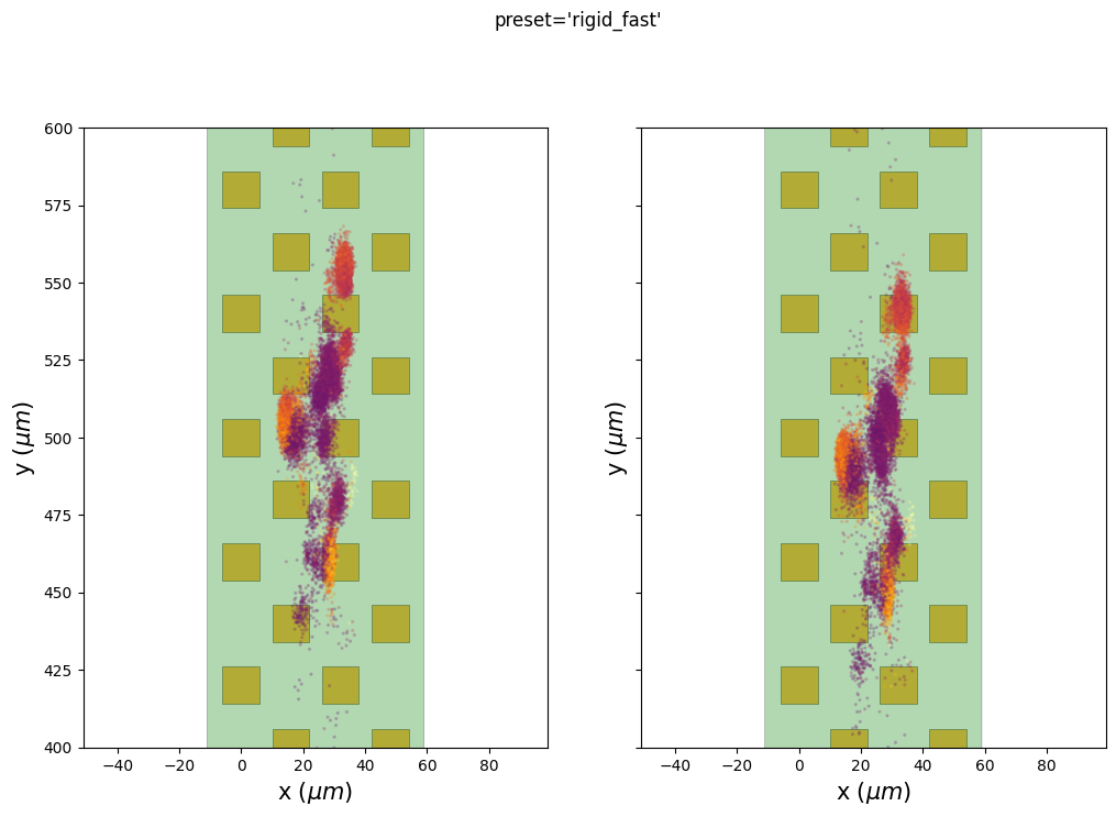

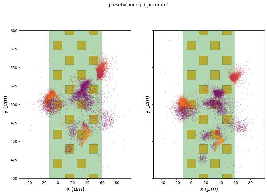
run times
Presets and related methods have different accuracies but also computation speeds. It is good to have this in mind!
run_times = []
for preset in some_presets:
    folder = base_folder / "motion_folder_dataset1" / preset
    motion_info = si.load_motion_info(folder)
    run_times.append(motion_info["run_times"])
keys = run_times[0].keys()

bottom = np.zeros(len(run_times))
fig, ax = plt.subplots(figsize=(14, 6))
for k in keys:
    rtimes = np.array([rt[k] for rt in run_times])
    if np.any(rtimes > 0.0):
        ax.bar(some_presets, rtimes, bottom=bottom, label=k)
    bottom += rtimes
ax.legend()
<matplotlib.legend.Legend at 0x7c9f003c1a90>