Note
Click here to download the full example code
Ground truth study tutorial
This tutorial illustrates how to run a “study”. A study is a systematic performance comparisons several ground truth recordings with several sorters.
The submodule study and the class propose high level tools functions to run many groundtruth comparison with many sorter on many recordings and then collect and aggregate results in an easy way.
The all mechanism is based on an intrinsinct organisation into a “study_folder” with several subfolder:
- raw_files : contain a copy in binary format of recordings
- sorter_folders : contains output of sorters
- ground_truth : contains a copy of sorting ground in npz format
- sortings: contains light copy of all sorting in npz format
- tables: some table in cvs format
In order to run and re run the computation all gt_sorting anf recordings are copied to a fast and universal format : binary (for recordings) and npz (for sortings).
Imports
import matplotlib.pyplot as plt
import seaborn as sns

import spikeinterface.extractors as se
import spikeinterface.widgets as sw
from spikeinterface.comparison import GroundTruthStudy
Setup study folder and run all sorters
We first generate the folder. this can take some time because recordings are copied inside the folder.
rec0, gt_sorting0 = se.example_datasets.toy_example(num_channels=4, duration=10, seed=10)
rec1, gt_sorting1 = se.example_datasets.toy_example(num_channels=4, duration=10, seed=0)
gt_dict = {
    'rec0': (rec0, gt_sorting0),
    'rec1': (rec1, gt_sorting1),
}
study_folder = 'a_study_folder'
study = GroundTruthStudy.create(study_folder, gt_dict)
Then just run all sorters on all recordings in one functions.
# sorter_list = st.sorters.available_sorters() # this get all sorters.
sorter_list = ['klusta', 'tridesclous', 'mountainsort4']
study.run_sorters(sorter_list, mode="keep")
Out:
RUNNING SHELL SCRIPT: /home/docs/checkouts/readthedocs.org/user_builds/spikeinterface/checkouts/0.13.0/examples/modules/comparison/a_study_folder/sorter_folders/rec0/klusta/run_klusta.sh
/home/docs/checkouts/readthedocs.org/user_builds/spikeinterface/checkouts/0.13.0/doc/sources/spikesorters/spikesorters/basesorter.py:158: ResourceWarning: unclosed file <_io.TextIOWrapper name=63 encoding='UTF-8'>
  self._run(recording, self.output_folders[i])
{'chunksize': 3000,
 'clean_cluster': {'apply_auto_merge_cluster': True,
                   'apply_auto_split': True,
                   'apply_trash_low_extremum': True,
                   'apply_trash_not_aligned': True,
                   'apply_trash_small_cluster': True},
 'clean_peaks': {'alien_value_threshold': None, 'mode': 'extremum_amplitude'},
 'cluster_kargs': {'adjacency_radius_um': 0.0,
                   'high_adjacency_radius_um': 0.0,
                   'max_loop': 1000,
                   'min_cluster_size': 20},
 'cluster_method': 'pruningshears',
 'duration': 10.0,
 'extract_waveforms': {'wf_left_ms': -2.0, 'wf_right_ms': 3.0},
 'feature_kargs': {'n_components': 8},
 'feature_method': 'global_pca',
 'make_catalogue': {'inter_sample_oversampling': False,
                    'sparse_thresh_level2': 3,
                    'subsample_ratio': 'auto'},
 'memory_mode': 'memmap',
 'mode': 'dense',
 'n_jobs': -1,
 'n_spike_for_centroid': 350,
 'noise_snippet': {'nb_snippet': 300},
 'peak_detector': {'adjacency_radius_um': 200.0,
                   'engine': 'numpy',
                   'method': 'global',
                   'peak_sign': '-',
                   'peak_span_ms': 0.7,
                   'relative_threshold': 5,
                   'smooth_radius_um': None},
 'peak_sampler': {'mode': 'rand', 'nb_max': 20000, 'nb_max_by_channel': None},
 'preprocessor': {'common_ref_removal': False,
                  'engine': 'numpy',
                  'highpass_freq': 400.0,
                  'lostfront_chunksize': -1,
                  'lowpass_freq': 5000.0,
                  'smooth_size': 0},
 'sparse_threshold': 1.5}
RUNNING SHELL SCRIPT: /home/docs/checkouts/readthedocs.org/user_builds/spikeinterface/checkouts/0.13.0/examples/modules/comparison/a_study_folder/sorter_folders/rec1/klusta/run_klusta.sh
/home/docs/checkouts/readthedocs.org/user_builds/spikeinterface/checkouts/0.13.0/doc/sources/spikesorters/spikesorters/basesorter.py:158: ResourceWarning: unclosed file <_io.TextIOWrapper name=63 encoding='UTF-8'>
  self._run(recording, self.output_folders[i])
{'chunksize': 3000,
 'clean_cluster': {'apply_auto_merge_cluster': True,
                   'apply_auto_split': True,
                   'apply_trash_low_extremum': True,
                   'apply_trash_not_aligned': True,
                   'apply_trash_small_cluster': True},
 'clean_peaks': {'alien_value_threshold': None, 'mode': 'extremum_amplitude'},
 'cluster_kargs': {'adjacency_radius_um': 0.0,
                   'high_adjacency_radius_um': 0.0,
                   'max_loop': 1000,
                   'min_cluster_size': 20},
 'cluster_method': 'pruningshears',
 'duration': 10.0,
 'extract_waveforms': {'wf_left_ms': -2.0, 'wf_right_ms': 3.0},
 'feature_kargs': {'n_components': 8},
 'feature_method': 'global_pca',
 'make_catalogue': {'inter_sample_oversampling': False,
                    'sparse_thresh_level2': 3,
                    'subsample_ratio': 'auto'},
 'memory_mode': 'memmap',
 'mode': 'dense',
 'n_jobs': -1,
 'n_spike_for_centroid': 350,
 'noise_snippet': {'nb_snippet': 300},
 'peak_detector': {'adjacency_radius_um': 200.0,
                   'engine': 'numpy',
                   'method': 'global',
                   'peak_sign': '-',
                   'peak_span_ms': 0.7,
                   'relative_threshold': 5,
                   'smooth_radius_um': None},
 'peak_sampler': {'mode': 'rand', 'nb_max': 20000, 'nb_max_by_channel': None},
 'preprocessor': {'common_ref_removal': False,
                  'engine': 'numpy',
                  'highpass_freq': 400.0,
                  'lostfront_chunksize': -1,
                  'lowpass_freq': 5000.0,
                  'smooth_size': 0},
 'sparse_threshold': 1.5}
You can re run run_study_sorters as many time as you want. By default mode=’keep’ so only uncomputed sorter are rerun. For instance, so just remove the “sorter_folders/rec1/herdingspikes” to re-run only one sorter on one recording.
Then we copy the spike sorting outputs into a separate subfolder. This allow to remove the “large” sorter_folders.
study.copy_sortings()
Collect comparisons
You can collect in one shot all results and run the GroundTruthComparison on it. So you can acces finely to all individual results.
Note that exhaustive_gt=True when you excatly how many units in ground truth (for synthetic datasets)
study.run_comparisons(exhaustive_gt=True)
for (rec_name, sorter_name), comp in study.comparisons.items():
print('*' * 10)
print(rec_name, sorter_name)
print(comp.count_score) # raw counting of tp/fp/...
comp.print_summary()
perf_unit = comp.get_performance(method='by_unit')
perf_avg = comp.get_performance(method='pooled_with_average')
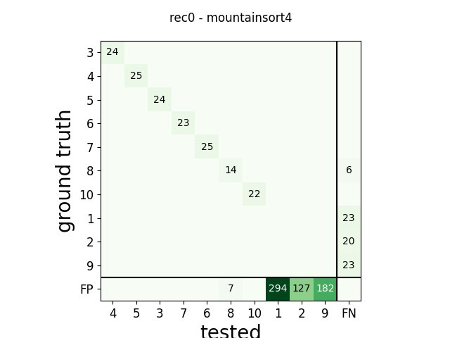
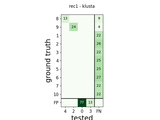
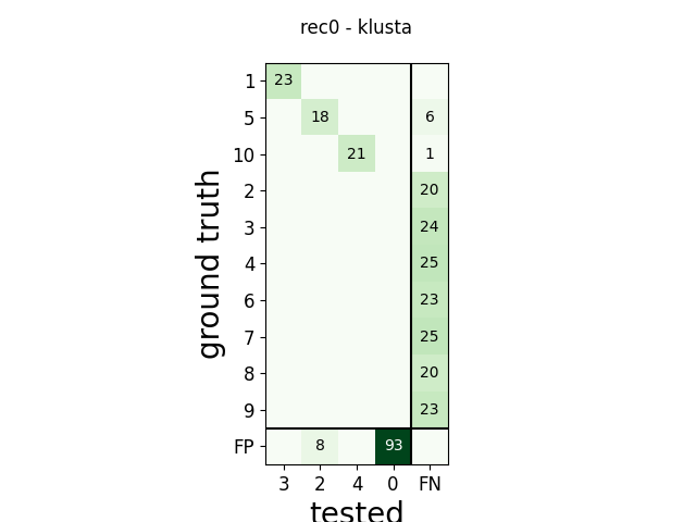
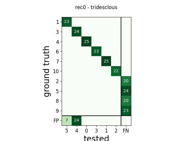
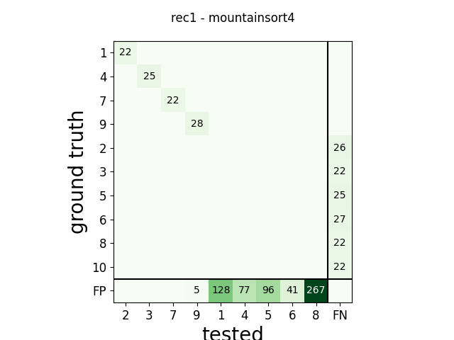
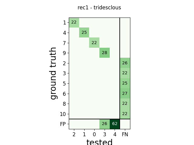
m = comp.get_confusion_matrix()
w_comp = sw.plot_confusion_matrix(comp)
w_comp.ax.set_title(rec_name + ' - ' + sorter_name)
Out:
**********
rec0 mountainsort4
            tp  fn fp num_gt num_tested tested_id
gt_unit_id
1            0  23  0     23          0        -1
2            0  20  0     20          0        -1
3           24   0  0     24         24         4
4           25   0  0     25         25         5
5           24   0  0     24         24         3
6           23   0  0     23         23         7
7           25   0  0     25         25         6
8           14   6  7     20         21         8
9            0  23  0     23          0        -1
10          22   0  0     22         22        10
SUMMARY
-------
GT num_units: 10
TESTED num_units: 10
num_well_detected: 6
num_redundant: 0
num_overmerged: 0
num_false_positive_units 3
num_bad: 3

**********
rec1 klusta
            tp  fn fp num_gt num_tested tested_id
gt_unit_id
1            0  22  0     22          0        -1
2            0  26  0     26          0        -1
3            0  22  0     22          0        -1
4            0  25  0     25          0        -1
5            0  25  0     25          0        -1
6            0  27  0     27          0        -1
7            0  22  0     22          0        -1
8           13   9  0     22         13         4
9           24   4  0     28         24         2
10           0  22  0     22          0        -1
SUMMARY
-------
GT num_units: 10
TESTED num_units: 4
num_well_detected: 1
num_redundant: 0
num_overmerged: 1
num_false_positive_units 0
num_bad: 2

**********
rec0 klusta
            tp  fn fp num_gt num_tested tested_id
gt_unit_id
1           23   0  0     23         23         3
2            0  20  0     20          0        -1
3            0  24  0     24          0        -1
4            0  25  0     25          0        -1
5           18   6  8     24         26         2
6            0  23  0     23          0        -1
7            0  25  0     25          0        -1
8            0  20  0     20          0        -1
9            0  23  0     23          0        -1
10          21   1  0     22         21         4
SUMMARY
-------
GT num_units: 10
TESTED num_units: 4
num_well_detected: 2
num_redundant: 0
num_overmerged: 1
num_false_positive_units 0
num_bad: 1

**********
rec0 tridesclous
            tp  fn  fp num_gt num_tested tested_id
gt_unit_id
1           23   0   7     23         30         5
2            0  20   0     20          0        -1
3           24   0  24     24         48         4
4           25   0   0     25         25         0
5            0  24   0     24          0        -1
6           23   0   0     23         23         3
7           25   0   0     25         25         1
8            0  20   0     20          0        -1
9            0  23   0     23          0        -1
10          22   0   0     22         22         2
SUMMARY
-------
GT num_units: 10
TESTED num_units: 6
num_well_detected: 4
num_redundant: 0
num_overmerged: 1
num_false_positive_units 0
num_bad: 0

**********
rec1 mountainsort4
            tp  fn fp num_gt num_tested tested_id
gt_unit_id
1           22   0  0     22         22         2
2            0  26  0     26          0        -1
3            0  22  0     22          0        -1
4           25   0  0     25         25         3
5            0  25  0     25          0        -1
6            0  27  0     27          0        -1
7           22   0  0     22         22         7
8            0  22  0     22          0        -1
9           28   0  5     28         33         9
10           0  22  0     22          0        -1
SUMMARY
-------
GT num_units: 10
TESTED num_units: 9
num_well_detected: 4
num_redundant: 0
num_overmerged: 2
num_false_positive_units 3
num_bad: 5

**********
rec1 tridesclous
            tp  fn  fp num_gt num_tested tested_id
gt_unit_id
1           22   0   0     22         22         2
2            0  26   0     26          0        -1
3            0  22   0     22          0        -1
4           25   0   0     25         25         1
5            0  25   0     25          0        -1
6            0  27   0     27          0        -1
7           22   0   0     22         22         0
8            0  22   0     22          0        -1
9           28   0  26     28         54         3
10           0  22   0     22          0        -1
SUMMARY
-------
GT num_units: 10
TESTED num_units: 5
num_well_detected: 3
num_redundant: 0
num_overmerged: 2
num_false_positive_units 0
num_bad: 1
Collect synthetic dataframes and display
As shown previously, the performance is returned as a pandas dataframe.
The aggregate_performances_table function, gathers all the outputs in
the study folder and merges them in a single dataframe.
dataframes = study.aggregate_dataframes()
Pandas dataframes can be nicely displayed as tables in the notebook.
print(dataframes.keys())
Out:
dict_keys(['run_times', 'perf_by_units', 'count_units'])
print(dataframes['run_times'])
Out:
  rec_name    sorter_name  run_time
0     rec1  mountainsort4  1.287447
1     rec1    tridesclous  1.425234
2     rec0    tridesclous  1.560422
3     rec0         klusta  1.943773
4     rec1         klusta  1.888482
5     rec0  mountainsort4  1.293365
Easy plot with seaborn
Seaborn allows to easily plot pandas dataframes. Let’s see some examples.
run_times = dataframes['run_times']
fig1, ax1 = plt.subplots()
sns.barplot(data=run_times, x='rec_name', y='run_time', hue='sorter_name', ax=ax1)
ax1.set_title('Run times')
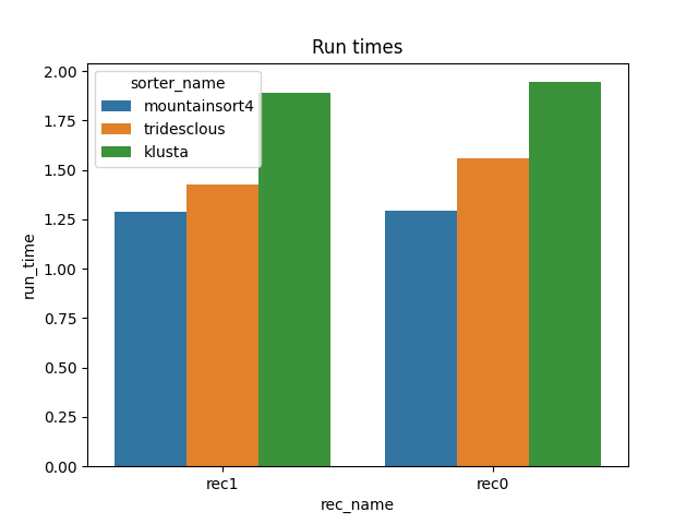
Out:
Text(0.5, 1.0, 'Run times')
perfs = dataframes['perf_by_units']
fig2, ax2 = plt.subplots()
sns.swarmplot(data=perfs, x='sorter_name', y='recall', hue='rec_name', ax=ax2)
ax2.set_title('Recall')
ax2.set_ylim(-0.1, 1.1)
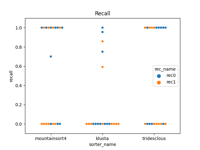
Out:
(-0.1, 1.1)
Total running time of the script: ( 0 minutes 11.485 seconds)