%matplotlib inline

How to “get started”¶

In this introductory example, you will see how to use the SpikeInterface to perform a full electrophysiology analysis. We will download simulated dataset, and we will then perform some pre-processing, run a spike sorting algorithm, post-process the spike sorting output, perform curation (manual and automatic), and compare spike sorting results.

import matplotlib.pyplot as plt
from pprint import pprint

The spikeinterface module by itself import only the spikeinterface.core submodule which is not useful for end user

import spikeinterface

We need to import one by one different submodules separately (preferred). There several modules:

extractors : file IO
preprocessing : preprocessing
sorters : Python wrappers of spike sorters
postprocessing : postprocessing
qualitymetrics : quality metrics on units found by sorter
curation : automatic curation of spike sorting output
comparison : comparison of spike sorting output
widgets : visualization

import spikeinterface as si  # import core only
import spikeinterface.extractors as se
import spikeinterface.preprocessing as spre
import spikeinterface.sorters as ss
import spikeinterface.postprocessing as spost
import spikeinterface.qualitymetrics as sqm
import spikeinterface.comparison as sc
import spikeinterface.exporters as sexp
import spikeinterface.curation as scur
import spikeinterface.widgets as sw

We can also import all submodules at once with this this internally import core+extractors+preprocessing+sorters+postprocessing+ qualitymetrics+comparison+widgets+exporters

This is useful for notebooks, but it is a heavier import because internally many more dependencies are imported (scipy/sklearn/networkx/matplotlib/h5py…)

import spikeinterface.full as si

Before getting started, we can set some global arguments for parallel processing. For this example, let’s use 4 jobs and time chunks of 1s:

global_job_kwargs = dict(n_jobs=4, chunk_duration="1s")
si.set_global_job_kwargs(**global_job_kwargs)

First, let’s download a simulated dataset from the https://gin.g-node.org/NeuralEnsemble/ephy_testing_data repo

Then we can open it. Note that MEArec simulated file contains both “recording” and a “sorting” object.

local_path = si.download_dataset(remote_path='mearec/mearec_test_10s.h5')
recording, sorting_true = se.read_mearec(local_path)
print(recording)
print(sorting_true)

MEArecRecordingExtractor: 32 channels - 1 segments - 32.0kHz - 10.000s
  file_path: /home/alessio/spikeinterface_datasets/ephy_testing_data/mearec/mearec_test_10s.h5
MEArecSortingExtractor: 10 units - 1 segments - 32.0kHz
  file_path: /home/alessio/spikeinterface_datasets/ephy_testing_data/mearec/mearec_test_10s.h5

recording is a BaseRecording object, which extracts information about channel ids, channel locations (if present), the sampling frequency of the recording, and the extracellular traces. sorting_true is a :BaseSorting object, which contains information about spike-sorting related information, including unit ids, spike trains, etc. Since the data are simulated, sorting_true has ground-truth information of the spiking activity of each unit.

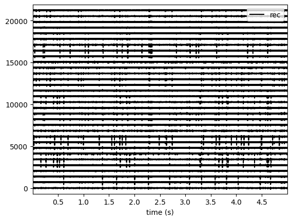
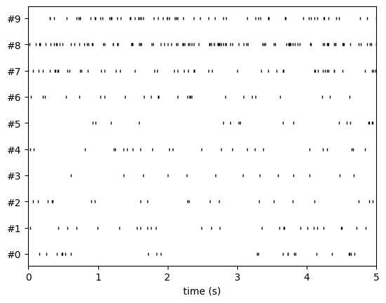
Let’s use the spikeinterface.widgets module to visualize the traces and the raster plots.

w_ts = sw.plot_timeseries(recording, time_range=(0, 5))
w_rs = sw.plot_rasters(sorting_true, time_range=(0, 5))

This is how you retrieve info from a BaseRecording…

channel_ids = recording.get_channel_ids()
fs = recording.get_sampling_frequency()
num_chan = recording.get_num_channels()
num_seg = recording.get_num_segments()

print('Channel ids:', channel_ids)
print('Sampling frequency:', fs)
print('Number of channels:', num_chan)
print('Number of segments:', num_seg)

Channel ids: ['1' '2' '3' '4' '5' '6' '7' '8' '9' '10' '11' '12' '13' '14' '15' '16'
 '17' '18' '19' '20' '21' '22' '23' '24' '25' '26' '27' '28' '29' '30'
 '31' '32']
Sampling frequency: 32000.0
Number of channels: 32
Number of segments: 1

…and a BaseSorting

num_seg = recording.get_num_segments()
unit_ids = sorting_true.get_unit_ids()
spike_train = sorting_true.get_unit_spike_train(unit_id=unit_ids[0])

print('Number of segments:', num_seg)
print('Unit ids:', unit_ids)
print('Spike train of first unit:', spike_train)

Number of segments: 1
Unit ids: ['#0' '#1' '#2' '#3' '#4' '#5' '#6' '#7' '#8' '#9']
Spike train of first unit: [  5197   8413  13124  15420  15497  15668  16929  19607  55107  59060
  60958 105193 105569 117082 119243 119326 122293 122877 132413 139498
 147402 147682 148271 149857 165454 170569 174319 176237 183598 192278
 201535 217193 219715 221226 222967 223897 225338 243206 243775 248754
 253184 253308 265132 266197 266662 283149 284716 287592 304025 305286
 310438 310775 318460]

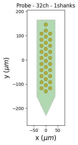
SpikeInterface internally uses the `ProbeInterface <https://probeinterface.readthedocs.io/en/main/>`__ to handle probeinterface.Probe and probeinterface.ProbeGroup. So any probe in the probeinterface collections can be downloaded and set to a Recording object. In this case, the MEArec dataset already handles a Probe and we don’t need to set it manually.

probe = recording.get_probe()
print(probe)

from probeinterface.plotting import plot_probe

_ = plot_probe(probe)

Probe - 32ch - 1shanks

Using the :spikeinterface.preprocessing, you can perform preprocessing on the recordings. Each pre-processing function also returns a BaseRecording, which makes it easy to build pipelines. Here, we filter the recording and apply common median reference (CMR). All these preprocessing steps are “lazy”. The computation is done on demand when we call recording.get_traces(...) or when we save the object to disk.

recording_cmr = recording
recording_f = si.bandpass_filter(recording, freq_min=300, freq_max=6000)
print(recording_f)
recording_cmr = si.common_reference(recording_f, reference='global', operator='median')
print(recording_cmr)

# this computes and saves the recording after applying the preprocessing chain
recording_preprocessed = recording_cmr.save(format='binary')
print(recording_preprocessed)

BandpassFilterRecording: 32 channels - 1 segments - 32.0kHz - 10.000s
CommonReferenceRecording: 32 channels - 1 segments - 32.0kHz - 10.000s
BinaryFolderRecording: 32 channels - 1 segments - 32.0kHz - 10.000s

Now you are ready to spike sort using the spikeinterface.sorters module! Let’s first check which sorters are implemented and which are installed

print('Available sorters', ss.available_sorters())
print('Installed sorters', ss.installed_sorters())

Available sorters ['combinato', 'hdsort', 'herdingspikes', 'ironclust', 'kilosort', 'kilosort2', 'kilosort2_5', 'kilosort3', 'klusta', 'mountainsort4', 'pykilosort', 'spykingcircus', 'spykingcircus2', 'tridesclous', 'tridesclous2', 'waveclus', 'waveclus_snippets', 'yass']
Installed sorters ['herdingspikes', 'kilosort2_5', 'mountainsort4', 'pykilosort', 'spykingcircus2', 'tridesclous', 'tridesclous2']

The ss.installed_sorters() will list the sorters installed in the machine. We can see we have HerdingSpikes and Tridesclous installed. Spike sorters come with a set of parameters that users can change. The available parameters are dictionaries and can be accessed with:

print("Tridesclous params:")
pprint(ss.get_default_sorter_params('tridesclous'))
print("SpykingCircus2 params:")
pprint(ss.get_default_sorter_params('spykingcircus2'))

Tridesclous params:
{'chunk_duration': '1s',
 'common_ref_removal': False,
 'detect_sign': -1,
 'detect_threshold': 5,
 'freq_max': 5000.0,
 'freq_min': 400.0,
 'n_jobs': 32,
 'nested_params': None,
 'progress_bar': True}
SpykingCircus2 params:
{'apply_preprocessing': True,
 'clustering': {},
 'detection': {'detect_threshold': 5, 'peak_sign': 'neg'},
 'filtering': {'dtype': 'float32'},
 'general': {'local_radius_um': 100, 'ms_after': 2, 'ms_before': 2},
 'job_kwargs': {},
 'localization': {},
 'matching': {},
 'registration': {},
 'selection': {'min_n_peaks': 20000, 'n_peaks_per_channel': 5000},
 'shared_memory': False,
 'waveforms': {'max_spikes_per_unit': 200, 'overwrite': True}}

Let’s run tridesclous and change one of the parameter, say, the detect_threshold:

sorting_TDC = ss.run_sorter(sorter_name="tridesclous", recording=recording_preprocessed, detect_threshold=4)
print(sorting_TDC)

TridesclousSortingExtractor: 10 units - 1 segments - 32.0kHz

Alternatively we can pass full dictionary containing the parameters:

other_params = ss.get_default_sorter_params('tridesclous')
other_params['detect_threshold'] = 6

# parameters set by params dictionary
sorting_TDC_2 = ss.run_sorter(sorter_name="tridesclous", recording=recording_preprocessed,
                              output_folder="tdc_output2", **other_params)
print(sorting_TDC_2)

TridesclousSortingExtractor: 9 units - 1 segments - 32.0kHz

Let’s run spykingcircus2 as well, with default parameters:

sorting_SC2 = ss.run_sorter(sorter_name="spykingcircus2", recording=recording_preprocessed)
print(sorting_SC2)

NpzFolderSorting: 10 units - 1 segments - 32.0kHz

The sorting_TDC and sorting_SC2 are BaseSorting objects. We can print the units found using:

print('Units found by tridesclous:', sorting_TDC.get_unit_ids())
print('Units found by spyking-circus2:', sorting_SC2.get_unit_ids())

Units found by tridesclous: [0 1 2 3 4 5 6 7 8 9]
Units found by spyking-circus2: [0 1 2 3 4 5 6 7 8 9]

If a sorter is not installed locally, we can also avoid to install it and run it anyways, using a container (Docker or Singularity). For example, let’s run Kilosort2 using Docker:

sorting_KS2 = ss.run_sorter(sorter_name="kilosort2", recording=recording_preprocessed,
                            docker_image=True, verbose=True)
print(sorting_KS2)

Starting container
Installing spikeinterface from sources in spikeinterface/kilosort2-compiled-base
Installing dev spikeinterface from local machine
Installing extra requirements: ['neo', 'mearec']
Running kilosort2 sorter inside spikeinterface/kilosort2-compiled-base
Stopping container

KiloSortSortingExtractor: 19 units - 1 segments - 32.0kHz

SpikeInterface provides a efficient way to extract waveforms from paired recording/sorting objects. The extract_waveforms function samples some spikes (by default max_spikes_per_unit=500) for each unit, extracts, their waveforms, and stores them to disk. These waveforms are helpful to compute the average waveform, or “template”, for each unit and then to compute, for example, quality metrics.

we_TDC = si.extract_waveforms(recording_preprocessed, sorting_TDC, 'waveforms_folder', overwrite=True)
print(we_TDC)

unit_id0 = sorting_TDC.unit_ids[0]
wavefroms = we_TDC.get_waveforms(unit_id0)
print(wavefroms.shape)

template = we_TDC.get_template(unit_id0)
print(template.shape)

WaveformExtractor: 32 channels - 10 units - 1 segments
  before:96 after:128 n_per_units:500
(30, 224, 32)
(224, 32)

we_TDC is a have the WaveformExtractor object we can post-process, validate, and curate the results. With the spikeinterface.postprocessing submodule, one can, for example, compute spike amplitudes, PCA projections, unit locations, and more.

Let’s compute some postprocessing information that will be needed later for computing quality metrics, exporting, and visualization:

amplitudes = spost.compute_spike_amplitudes(we_TDC)
unit_locations = spost.compute_unit_locations(we_TDC)
spike_locations = spost.compute_spike_locations(we_TDC)
correlograms, bins = spost.compute_correlograms(we_TDC)
similarity = spost.compute_template_similarity(we_TDC)

All of this postprocessing functions are saved in the waveforms folder as extensions:

print(we_TDC.get_available_extension_names())

['similarity', 'spike_amplitudes', 'correlograms', 'spike_locations', 'unit_locations']

Importantly, waveform extractors (and all extensions) can be reloaded at later times:

we_loaded = si.load_waveforms('waveforms_folder')
print(we_loaded.get_available_extension_names())

['similarity', 'spike_amplitudes', 'correlograms', 'spike_locations', 'unit_locations']

Once we have computed all these postprocessing information, we can compute quality metrics (different quality metrics require different extensions - e.g., drift metrics resuire spike_locations):

qm_params = sqm.get_default_qm_params()
pprint(qm_params)

{'amplitude_cutoff': {'amplitudes_bins_min_ratio': 5,
                      'histogram_smoothing_value': 3,
                      'num_histogram_bins': 100,
                      'peak_sign': 'neg'},
 'amplitude_median': {'peak_sign': 'neg'},
 'drift': {'direction': 'y',
           'interval_s': 60,
           'min_num_bins': 2,
           'min_spikes_per_interval': 100},
 'isi_violation': {'isi_threshold_ms': 1.5, 'min_isi_ms': 0},
 'nearest_neighbor': {'max_spikes': 10000, 'n_neighbors': 5},
 'nn_isolation': {'max_spikes': 10000,
                  'min_spikes': 10,
                  'n_components': 10,
                  'n_neighbors': 4,
                  'peak_sign': 'neg',
                  'radius_um': 100},
 'nn_noise_overlap': {'max_spikes': 10000,
                      'min_spikes': 10,
                      'n_components': 10,
                      'n_neighbors': 4,
                      'peak_sign': 'neg',
                      'radius_um': 100},
 'presence_ratio': {'bin_duration_s': 60},
 'rp_violation': {'censored_period_ms': 0.0, 'refractory_period_ms': 1.0},
 'sliding_rp_violation': {'bin_size_ms': 0.25,
                          'contamination_values': None,
                          'exclude_ref_period_below_ms': 0.5,
                          'max_ref_period_ms': 10,
                          'window_size_s': 1},
 'snr': {'peak_mode': 'extremum',
         'peak_sign': 'neg',
         'random_chunk_kwargs_dict': None}}

Since the recording is very short, let’s change some parameters to accomodate the duration:

qm_params["presence_ratio"]["bin_duration_s"] = 1
qm_params["amplitude_cutoff"]["num_histogram_bins"] = 5
qm_params["drift"]["interval_s"] = 2
qm_params["drift"]["min_spikes_per_interval"] = 2

qm = sqm.compute_quality_metrics(we_TDC, qm_params=qm_params)
display(qm)

	num_spikes	firing_rate	presence_ratio	snr	sliding_rp_violation	amplitude_cutoff	amplitude_median	drift_ptp	drift_std	drift_mad
0	30	3.0	0.9	27.258799	NaN	0.200717	307.199036	1.313088	0.492143	0.476104
1	51	5.1	1.0	24.213808	NaN	0.500000	274.444977	0.934371	0.325045	0.216362
2	53	5.3	0.9	24.229277	NaN	0.500000	270.204590	0.901922	0.392344	0.372247
3	50	5.0	1.0	27.080778	NaN	0.500000	312.545715	0.598991	0.225554	0.185147
4	36	3.6	1.0	9.544292	NaN	0.207231	107.953278	1.913661	0.659317	0.507955
5	42	4.2	1.0	13.283191	NaN	0.204838	151.833191	0.671453	0.231825	0.156004
6	48	4.8	1.0	8.319447	NaN	0.500000	91.358444	2.391275	0.885580	0.772367
7	193	19.3	1.0	8.690839	0.155	0.500000	103.491577	0.710640	0.300565	0.316645
8	129	12.9	1.0	11.167040	0.310	0.500000	128.252319	0.985251	0.375529	0.301622
9	110	11.0	1.0	8.377251	0.270	0.203415	98.207291	1.386857	0.526532	0.410644

Quality metrics are also extensions (and become part of the waveform folder):

Next, we can use some of the powerful tools for spike sorting visualization.

We can export a sorting summary and quality metrics plot using the sortingview backend. This will generate shareble links for web-based visualization.

w1 = sw.plot_quality_metrics(we_TDC, display=False, backend="sortingview")

https://figurl.org/f?v=gs://figurl/spikesortingview-10&d=sha1://901a11ba31ae9ab512a99bdf36a3874173249d87&label=SpikeInterface%20-%20Quality%20Metrics

w2 = sw.plot_sorting_summary(we_TDC, display=False, curation=True, backend="sortingview")

https://figurl.org/f?v=gs://figurl/spikesortingview-10&d=sha1://cd190c64eeea6a0ceaf57d1153b6ab4eac351d70&label=SpikeInterface%20-%20Sorting%20Summary

The sorting summary plot can also be used for manual labeling and curation. In the example above, we manually merged two units (0, 4) and added accept labels (2, 6, 7). After applying our curation, we can click on the “Save as snapshot (sha://)” and copy the URI:

uri = "sha1://68cb54a9aaed2303fb82dedbc302c853e818f1b6"

sorting_curated_sv = scur.apply_sortingview_curation(sorting_TDC, uri_or_json=uri)
print(sorting_curated_sv)
print(sorting_curated_sv.get_property("accept"))

MergeUnitsSorting: 9 units - 1 segments - 32.0kHz
[False  True False False  True  True False False False]

Alternatively, we can export the data locally to Phy. Phy is a GUI for manual curation of the spike sorting output. To export to phy you can run:

sexp.export_to_phy(we_TDC, 'phy_folder_for_TDC', verbose=True)

Run:
phy template-gui  /home/alessio/Documents/codes/spike_sorting/spikeinterface/spikeinterface/examples/how_to/phy_folder_for_TDC/params.py

Then you can run the template-gui with: phy template-gui phy_folder_for_TDC/params.py and manually curate the results.

After curating with Phy, the curated sorting can be reloaded to SpikeInterface. In this case, we exclude the units that have been labeled as “noise”:

sorting_curated_phy = se.read_phy('phy_folder_for_TDC', exclude_cluster_groups=["noise"])

Quality metrics can be also used to automatically curate the spike sorting output. For example, you can select sorted units with a SNR above a certain threshold:

keep_mask = (qm['snr'] > 10) & (qm['isi_violations_ratio'] < 0.01)
print("Mask:", keep_mask.values)

sorting_curated_auto = sorting_TDC.select_units(sorting_TDC.unit_ids[keep_mask])
print(sorting_curated_auto)

Mask: [ True  True  True  True False  True False False  True False]
UnitsSelectionSorting: 6 units - 1 segments - 32.0kHz

The final part of this tutorial deals with comparing spike sorting outputs. We can either:

compare the spike sorting results with the ground-truth sorting sorting_true
compare the output of two (Tridesclous and SpykingCircus2)
compare the output of multiple sorters (Tridesclous, SpykingCircus2, Kilosort2)

comp_gt = sc.compare_sorter_to_ground_truth(gt_sorting=sorting_true, tested_sorting=sorting_TDC)
comp_pair = sc.compare_two_sorters(sorting1=sorting_TDC, sorting2=sorting_SC2)
comp_multi = sc.compare_multiple_sorters(sorting_list=[sorting_TDC, sorting_SC2, sorting_KS2],
                                         name_list=['tdc', 'sc2', 'ks2'])

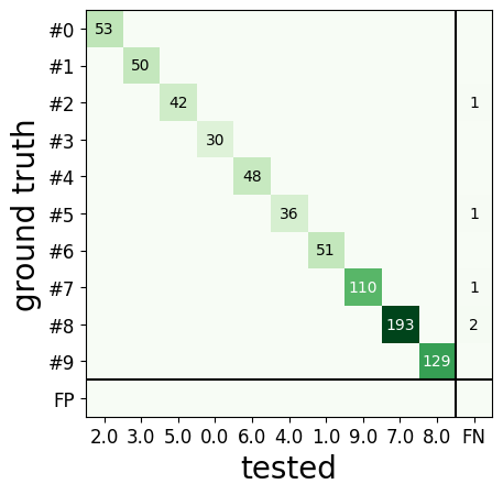
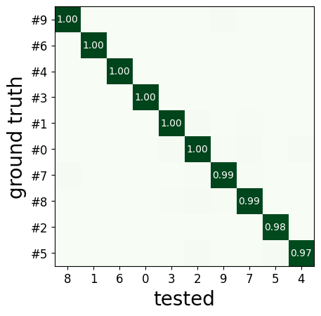
When comparing with a ground-truth sorting (1,), you can get the sorting performance and plot a confusion matrix

print(comp_gt.get_performance())
w_conf = sw.plot_confusion_matrix(comp_gt)
w_agr = sw.plot_agreement_matrix(comp_gt)

            accuracy    recall precision false_discovery_rate miss_rate
gt_unit_id
#0               1.0       1.0       1.0                  0.0       0.0
#1               1.0       1.0       1.0                  0.0       0.0
#2          0.976744  0.976744       1.0                  0.0  0.023256
#3               1.0       1.0       1.0                  0.0       0.0
#4               1.0       1.0       1.0                  0.0       0.0
#5          0.972973  0.972973       1.0                  0.0  0.027027
#6               1.0       1.0       1.0                  0.0       0.0
#7          0.990991  0.990991       1.0                  0.0  0.009009
#8          0.989744  0.989744       1.0                  0.0  0.010256
#9               1.0       1.0       1.0                  0.0       0.0

When comparing two sorters (2.), we can see the matching of units between sorters. Units which are not matched has -1 as unit id:

comp_pair.hungarian_match_12

or the reverse:

comp_pair.hungarian_match_21

When comparing multiple sorters (3.), you can extract a BaseSorting object with units in agreement between sorters. You can also plot a graph showing how the units are matched between the sorters.

sorting_agreement = comp_multi.get_agreement_sorting(minimum_agreement_count=2)

print('Units in agreement between TDC, SC2, and KS2:', sorting_agreement.get_unit_ids())

w_multi = sw.plot_multicomp_agreement(comp_multi)
w_multi = sw.plot_multicomp_agreement_by_sorter(comp_multi)

Units in agreement between TDC, SC2, and KS2: [0 1 2 3 4 5 6 7 8 9]

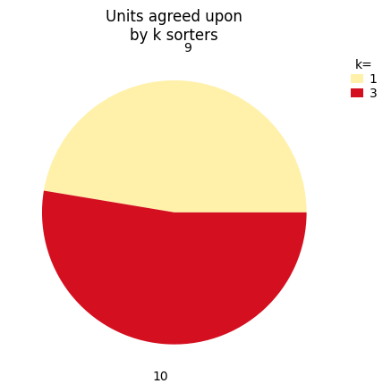
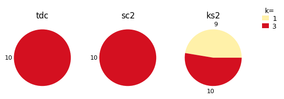
We see that 10 unit were found by all sorters (note that this simulated dataset is a very simple example, and usually sorters do not do such a great job)!

However, Kilosort2 found 9 additional units that are not matched to ground-truth!

That’s all for this “How to get started” tutorial! Enjoy SpikeInterface!