Inter-spike-interval (ISI) violations (`isi_violation`)¶

Calculation¶

Neurons have a refractory period after a spiking event during which they cannot fire again. Inter-spike-interval (ISI) violations refers to the rate of refractory period violations (as described by Hill).

The calculation works under the assumption that the contaminant events happen randomly, or comes from another neuron that is not correlated with our unit. A correlation will lead to an over-estimation of the contamination, whereas an anti-correlation will lead to an under-estimation.

Different formulas were developped over the years.

Calculation from the Hill paper¶

The following quantities are required:

\(ISI_t\) : biological threshold for ISI violation.
\(ISI_{min}\): minimum ISI threshold enforced by the data recording system used.
\(ISI_s\) : the array of ISI violations which are observed in the unit’s spike train.
\(\#\): denote count.

The threshold for ISI violations is the biological ISI threshold, \(ISI_t\), minus the minimum ISI threshold, \(ISI_{min}\) enforced by the data recording system used. The array of inter-spike-intervals observed in the unit’s spike train, \(ISI_s\), is used to identify the count (\(\#\)) of observed ISI’s below this threshold. For a recording with a duration of \(T_r\) seconds, and a unit with \(N_s\) spikes, the rate of ISI violations is:

\[\textrm{ISI violations} = \frac{ \#( ISI_s < ISI_t) T_r }{ 2 N_s^2 (ISI_t - ISI_{min}) }\]

Calculation from the Llobet paper¶

The following quantities are required:

\(T\) the duration of the recording.
\(N\) the number of spikes in the unit’s spike train.
\(t_r\) the duration of the unit’s refractory period.
\(n_v\) the number of violations of the refractory period.

The estimated contamination \(C\) can be calculated with 2 extreme scenarios. In the first one, the contaminant spikes are completely random (or come from an infinite number of other neurons). In the second one, the contaminant spikes come from a single other neuron:

\[\begin{split}C = \frac{FP}{TP + FP} \approx \begin{cases} 1 - \sqrt{1 - \frac{n_v T}{N^2 t_r}} \text{ for the case of random contamination} \\ \frac{1}{2} \left( 1 - \sqrt{1 - \frac{2 n_v T}{N^2 t_r}} \right) \text{ for the case of 1 contaminant neuron} \end{cases}\end{split}\]

Where \(TP\) is the number of true positives (detected spikes that come from the neuron) and \(FP\) is the number of false positives (detected spikes that don’t come from the neuron).

Expectation and use¶

ISI violations identifies unit contamination - a high value indicates a highly contaminated unit. Despite being a ratio, ISI violations can exceed 1 (or become a complex number in the Llobet formula). This is usually due to the contaminant events being correlated with our neuron, and their number are greater than a purely random spike train.

Example code¶

Without SpikeInterface:

spike_train = ...   # The spike train of our unit
t_r = ...           # The refractory period of our unit
n_v = np.sum(np.diff(spike_train) < t_r)

# Use the formula you want here

With SpikeInterface:

import spikeinterface.qualitymetrics as qm

# Make recording, sorting and wvf_extractor object for your data.

isi_violations_ratio, isi_violations_rate, isi_violations_count = qm.compute_isi_violations(wvf_extractor, isi_threshold_ms=1.0)

References¶

Various cluster quality metrics.

Some of then come from or the old implementation: * https://github.com/AllenInstitute/ecephys_spike_sorting/tree/master/ecephys_spike_sorting/modules/quality_metrics * https://github.com/SpikeInterface/spikemetrics

Implementations here have been refactored to support the multi-segment API of spikeinterface.

spikeinterface.qualitymetrics.misc_metrics.compute_isi_violations(waveform_extractor, isi_threshold_ms=1.5, min_isi_ms=0, **kwargs)¶

Calculate Inter-Spike Interval (ISI) violations.

It computes several metrics related to isi violations:

isi_violations_ratio: the relative firing rate of the hypothetical neurons that are
generating the ISI violations. Described in [1]. See Notes.
isi_violation_rate: number of ISI violations divided by total rate
isi_violation_count: number of ISI violations

Parameters

waveform_extractorWaveformExtractor: The waveform extractor object
isi_threshold_msfloat, optional, default: 1.5: Threshold for classifying adjacent spikes as an ISI violation, in ms. This is the biophysical refractory period (default=1.5).
min_isi_msfloat, optional, default: 0: Minimum possible inter-spike interval, in ms. This is the artificial refractory period enforced by the data acquisition system or post-processing algorithms.

Returns

isi_violations_ratiofloat: The isi violation ratio described in [1].
isi_violations_ratefloat: Rate of contaminating spikes as a fraction of overall rate. Higher values indicate more contamination.
isi_violation_countint: Number of violations.

Notes

You can interpret an ISI violations ratio value of 0.5 as meaning that contaminating spikes are occurring at roughly half the rate of “true” spikes for that unit. In cases of highly contaminated units, the ISI violations ratio can sometimes be greater than 1.

Links to source code¶

From SpikeInterface

From Lussac

From the AllenSDK

Examples with plots¶

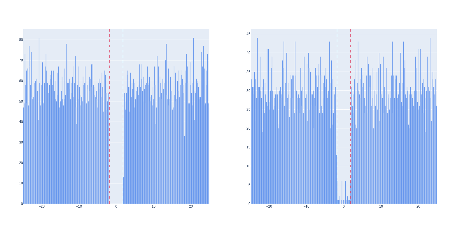
Here is shown the auto-correlogram of two units, with the dashed lines representing the refractory period.

On the left, we have a unit with no refractory period violations, meaning that this unit is probably not contaminated.
On the right, we have a unit with some refractory period violations. It means that it is contaminated, but probably not that much.

This figure can be generated with the following code:

import plotly.graph_objects as go
from spikeinterface.postprocessing import compute_correlograms

# Create your sorting object
unit_ids = ... # Units you are interested in vizulazing.
sorting = sorting.select_units(unit_ids)
t_r = 1.5   # Refractory period (in ms).

correlograms, bins = compute_correlograms(sorting, window_ms=50.0, bin_ms=0.2, symmetrize=True)

fig = go.Figure().set_subplots(rows=1, cols=2)

fig.add_trace(go.Bar(
    x=bins[:-1] + (bins[1]-bins[0])/2,
    y=correlograms[0, 0],
    width=bins[1] - bins[0],
    marker_color="CornflowerBlue",
    name="Non-contaminated unit",
    showlegend=False
), row=1, col=1)
fig.add_trace(go.Bar(
    x=bins[:-1] + (bins[1]-bins[0])/2,
    y=correlograms[1, 1],
    width=bins[1] - bins[0],
    marker_color="CornflowerBlue",
    name="Contaminated unit",
    showlegend=False
), row=1, col=2)

fig.add_vline(x=-t_r, row=1, col=1, line=dict(dash="dash", color="Crimson", width=1))
fig.add_vline(x=t_r, row=1, col=1, line=dict(dash="dash", color="Crimson", width=1))
fig.add_vline(x=-t_r, row=1, col=2, line=dict(dash="dash", color="Crimson", width=1))
fig.add_vline(x=t_r, row=1, col=2, line=dict(dash="dash", color="Crimson", width=1))

fig.show()

Literature¶

Introduced by [Hill] (2011).

Hill: Hill, Daniel N., Samar B. Mehta, and David Kleinfeld. “Quality Metrics to Accompany Spike Sorting of Extracellular Signals.” The Journal of neuroscience 31.24 (2011): 8699–8705. Web.

Also described by [Llobet] (2022)

Llobet: Llobet Victor, Wyngaard Aurélien and Barbour Boris. “Automatic post-processing and merging of multiple spike-sorting analyses with Lussac“. BioRxiv (2022).

Inter-spike-interval (ISI) violations (isi_violation)¶