Preprocessing Tutorial

Before spike sorting, you may need to preproccess your signals in order to improve the spike sorting performance. You can do that in SpikeInterface using the spikeinterface.preprocessing submodule.

import numpy as np
import matplotlib.pylab as plt
import scipy.signal

import spikeinterface.extractors as se
from spikeinterface.preprocessing import (bandpass_filter, notch_filter, common_reference,
                                          remove_artifacts, preprocesser_dict)

First, let’s create a toy example:

recording, sorting = se.toy_example(num_channels=4, duration=10, seed=0)

Apply filters

Now apply a bandpass filter and a notch filter (separately) to the recording extractor. Filters are also BaseRecording objects. Note that these operation are lazy the computation is done on the fly with rec.get_traces()

recording_bp = bandpass_filter(recording, freq_min=300, freq_max=6000)
print(recording_bp)
recording_notch = notch_filter(recording, freq=2000, q=30)
print(recording_notch)

BandpassFilterRecording: 4 channels - 2 segments - 30.0kHz - 20.000s
NotchFilterRecording: 4 channels - 2 segments - 30.0kHz - 20.000s

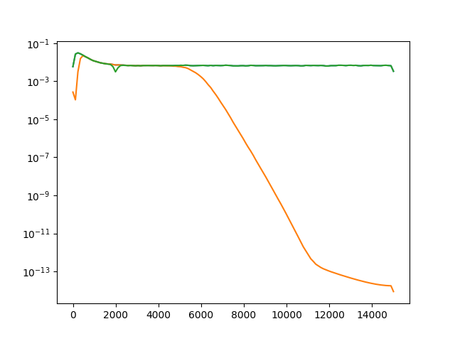
Now let’s plot the power spectrum of non-filtered, bandpass filtered, and notch filtered recordings.

fs = recording.get_sampling_frequency()

f_raw, p_raw = scipy.signal.welch(recording.get_traces(segment_index=0)[:, 0], fs=fs)
f_bp, p_bp = scipy.signal.welch(recording_bp.get_traces(segment_index=0)[:, 0], fs=fs)
f_notch, p_notch = scipy.signal.welch(recording_notch.get_traces(segment_index=0)[:, 0], fs=fs)

fig, ax = plt.subplots()
ax.semilogy(f_raw, p_raw, f_bp, p_bp, f_notch, p_notch)

[<matplotlib.lines.Line2D object at 0x7f2978211430>, <matplotlib.lines.Line2D object at 0x7f2978211190>, <matplotlib.lines.Line2D object at 0x7f29782115e0>]

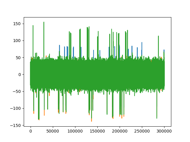
Change reference

In many cases, before spike sorting, it is wise to re-reference the signals to reduce the common-mode noise from the recordings.

To re-reference in spikeinterface.preprocessing you can use the common_reference() function. Both common average reference (CAR) and common median reference (CMR) can be applied. Moreover, the average/median can be computed on different groups. Single channels can also be used as reference.

recording_car = common_reference(recording, reference='global', operator='average')
recording_cmr = common_reference(recording, reference='global', operator='median')
recording_single = common_reference(recording, reference='single', ref_channel_ids=[1])
recording_single_groups = common_reference(recording, reference='single',
                                              groups=[[0, 1], [2, 3]],
                                              ref_channel_ids=[0, 2])


trace0_car = recording_car.get_traces(segment_index=0)[:, 0]
trace0_cmr = recording_cmr.get_traces(segment_index=0)[:, 0]
trace0_single = recording_single.get_traces(segment_index=0)[:, 0]
fig1, ax1 = plt.subplots()
ax1.plot(trace0_car)
ax1.plot(trace0_cmr)
ax1.plot(trace0_single)

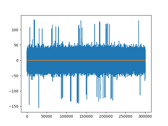
trace1_groups = recording_single_groups.get_traces(segment_index=0)[:, 1]
trace0_groups = recording_single_groups.get_traces(segment_index=0)[:, 0]
fig2, ax2 = plt.subplots()
ax2.plot(trace1_groups)  # not zero
ax2.plot(trace0_groups)

• 
• 

[<matplotlib.lines.Line2D object at 0x7f297801e1c0>]

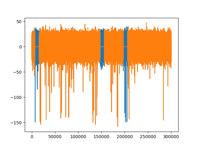
Remove stimulation artifacts

In some applications, electrodes are used to electrically stimulate the tissue, generating a large artifact. In spikeinterface.preprocessing, the artifact can be zeroed-out using the remove_artifacts() function.

# create dummy stimulation triggers per segment
stimulation_trigger_frames = [
        [10000, 150000, 200000],
        [20000, 30000],
    ]


# large ms_before and s_after are used for plotting only
recording_rm_artifact = remove_artifacts(recording, stimulation_trigger_frames,
                                                         ms_before=100, ms_after=200)

trace0 = recording.get_traces(segment_index=0)[:, 0]
trace0_rm = recording_rm_artifact.get_traces(segment_index=0)[:, 0]
fig3, ax3 = plt.subplots()
ax3.plot(trace0)
ax3.plot(trace0_rm)

[<matplotlib.lines.Line2D object at 0x7f29b0a49130>]

You can list the available preprocessors with:

from pprint import pprint
pprint(preprocesser_dict)


plt.show()

{'bandpass_filter': <class 'spikeinterface.preprocessing.filter.BandpassFilterRecording'>,
 'blank_staturation': <class 'spikeinterface.preprocessing.clip.BlankSaturationRecording'>,
 'center': <class 'spikeinterface.preprocessing.normalize_scale.ZScoreRecording'>,
 'clip': <class 'spikeinterface.preprocessing.clip.ClipRecording'>,
 'common_reference': <class 'spikeinterface.preprocessing.common_reference.CommonReferenceRecording'>,
 'deepinterpolate': <class 'spikeinterface.preprocessing.deepinterpolation.deepinterpolation.DeepInterpolatedRecording'>,
 'filter': <class 'spikeinterface.preprocessing.filter.FilterRecording'>,
 'highpass_filter': <class 'spikeinterface.preprocessing.filter.HighpassFilterRecording'>,
 'normalize_by_quantile': <class 'spikeinterface.preprocessing.normalize_scale.NormalizeByQuantileRecording'>,
 'notch_filter': <class 'spikeinterface.preprocessing.filter.NotchFilterRecording'>,
 'phase_shift': <class 'spikeinterface.preprocessing.phase_shift.PhaseShiftRecording'>,
 'rectify': <class 'spikeinterface.preprocessing.rectify.RectifyRecording'>,
 'remove_artifacts': <class 'spikeinterface.preprocessing.remove_artifacts.RemoveArtifactsRecording'>,
 'remove_bad_channels': <class 'spikeinterface.preprocessing.remove_bad_channels.RemoveBadChannelsRecording'>,
 'resample': <class 'spikeinterface.preprocessing.resample.ResampleRecording'>,
 'scale': <class 'spikeinterface.preprocessing.normalize_scale.ScaleRecording'>,
 'whiten': <class 'spikeinterface.preprocessing.whiten.WhitenRecording'>,
 'zero_channel_pad': <class 'spikeinterface.preprocessing.zero_channel_pad.ZeroChannelPaddedRecording'>}