Postprocessing Tutorial

Spike sorters generally output a set of units with corresponding spike trains. The postprocessing submodule allows to combine the RecordingExtractor and the sorted SortingExtractor objects to perform further postprocessing.

import matplotlib.pylab as plt

import spikeinterface as si
import spikeinterface.extractors as se
from spikeinterface.postprocessing import get_template_extremum_channel, compute_principal_components

First, let’s download a simulated dataset from the repo ‘https://gin.g-node.org/NeuralEnsemble/ephy_testing_data’

local_path = si.download_dataset(remote_path='mearec/mearec_test_10s.h5')
recording, sorting = se.read_mearec(local_path)
print(recording)
print(sorting)

MEArecRecordingExtractor: 32 channels - 1 segments - 32.0kHz - 10.000s
  file_path: /home/docs/spikeinterface_datasets/ephy_testing_data/mearec/mearec_test_10s.h5
MEArecSortingExtractor: 10 units - 1 segments - 32.0kHz
  file_path: /home/docs/spikeinterface_datasets/ephy_testing_data/mearec/mearec_test_10s.h5

Assuming the sorting is the output of a spike sorter, the postprocessing module allows to extract all relevant information from the paired recording-sorting.

Compute spike waveforms

Waveforms are extracted with the WaveformExtractor or directly with the extract_waveforms function (which returns a WaveformExtractor object):

folder = 'waveforms_mearec'
we = si.extract_waveforms(recording, sorting, folder,
                          load_if_exists=True,
                          ms_before=1, ms_after=2., max_spikes_per_unit=500,
                          n_jobs=1, chunk_size=30000)
print(we)

WaveformExtractor: 32 channels - 10 units - 1 segments
  before:32 after:64 n_per_units:500

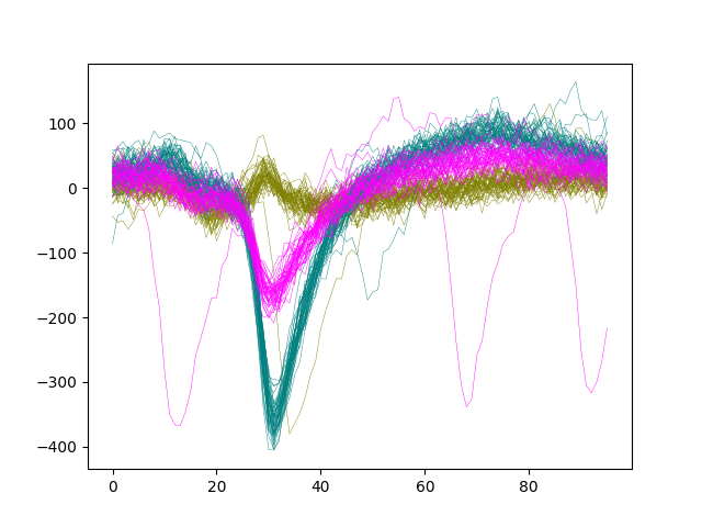
Let’s plot the waveforms of units [0, 1, 2] on channel 8

colors = ['Olive', 'Teal', 'Fuchsia']

fig, ax = plt.subplots()
for i, unit_id in enumerate(sorting.unit_ids[:3]):
    wf = we.get_waveforms(unit_id)
    color = colors[i]
    ax.plot(wf[:, :, 8].T, color=color, lw=0.3)

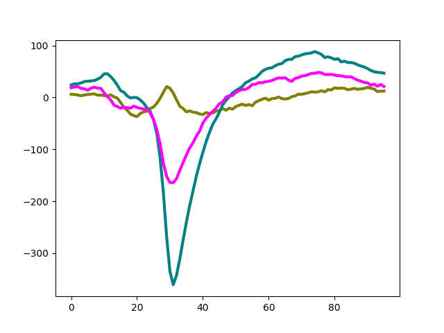
Compute unit templates

Similarly to waveforms, templates - average waveforms - can be easily retrieved from the WaveformExtractor object:

fig, ax = plt.subplots()
for i, unit_id in enumerate(sorting.unit_ids[:3]):
    template = we.get_template(unit_id)
    color = colors[i]
    ax.plot(template[:, 8].T, color=color, lw=3)

Compute unit maximum channel

In a similar way, one can get the recording channel with the ‘extremum’ signal (minimum or maximum). The code:get_template_extremum_channel outputs a dictionary unit_ids as keys and channel_ids as values:

extremum_channels_ids = get_template_extremum_channel(we, peak_sign='neg')
print(extremum_channels_ids)

{'#0': '6', '#1': '10', '#2': '20', '#3': '3', '#4': '15', '#5': '13', '#6': '25', '#7': '22', '#8': '23', '#9': '7'}

Compute principal components (aka PCs)

Computing PCA scores for each waveforms is very common for many applications, including unsupervised validation of the spike sorting performance.

There are different ways to compute PC scores from waveforms:

• “concatenated”: all waveforms are concatenated and a single PCA model is computed (channel information is lost)

• “by_channel_global”: PCA is computed from a subset of all waveforms and applied independently on each channel

• “by_channel_local”: PCA is computed and applied to each channel separately

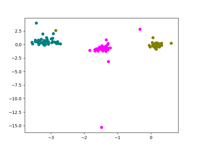
In SI, we can compute PC scores with the compute_principal_components function (which returns a WaveformPrincipalComponent object). The pc scores for a unit are retrieved with the get_projections function and the shape of the pc scores is (n_spikes, n_components, n_channels). Here, we compute PC scores and plot the first and second components of channel 8:

pc = compute_principal_components(we, load_if_exists=True,
                                  n_components=3, mode='by_channel_local')
print(pc)

fig, ax = plt.subplots()
for i, unit_id in enumerate(sorting.unit_ids[:3]):
    comp = pc.get_projections(unit_id)
    print(comp.shape)
    color = colors[i]
    ax.scatter(comp[:, 0, 8], comp[:, 1, 8], color=color)

WaveformPrincipalComponent: 32 channels - 1 segments
  mode:by_channel_local n_components:3
(53, 3, 32)
(50, 3, 32)
(43, 3, 32)

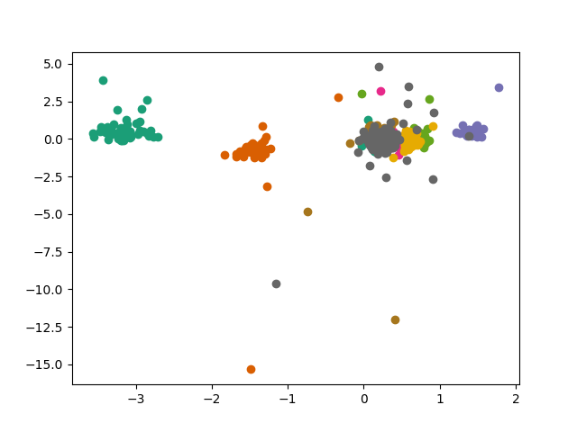
Note that PC scores for all units can be retrieved at once with the get_all_projections() function:

all_labels, all_projections = pc.get_all_projections()
print(all_labels[:40])
print(all_labels.shape)
print(all_projections.shape)

cmap = plt.get_cmap('Dark2', len(sorting.unit_ids))

fig, ax = plt.subplots()
for i, unit_id in enumerate(sorting.unit_ids):
    mask = all_labels == unit_id
    comp = all_projections[mask, :, :]
    ax.scatter(comp[:, 0, 8], comp[:, 1, 8], color=cmap(i))

plt.show()

['#0' '#0' '#0' '#0' '#0' '#0' '#0' '#0' '#0' '#0' '#0' '#0' '#0' '#0'
 '#0' '#0' '#0' '#0' '#0' '#0' '#0' '#0' '#0' '#0' '#0' '#0' '#0' '#0'
 '#0' '#0' '#0' '#0' '#0' '#0' '#0' '#0' '#0' '#0' '#0' '#0']
(745,)
(745, 3, 32)