RecordingExtractor Widgets Gallery

Here is a gallery of all the available widgets using RecordingExtractor objects.

import matplotlib.pyplot as plt

import spikeinterface.extractors as se
import spikeinterface.widgets as sw

First, let’s create a toy example with the extractors module:

recording, sorting = se.toy_example(duration=10, num_channels=4, seed=0, num_segments=1)

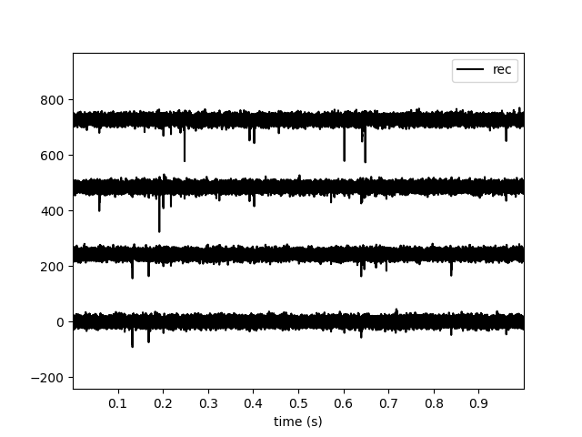
plot_timeseries()

w_ts = sw.plot_timeseries(recording)

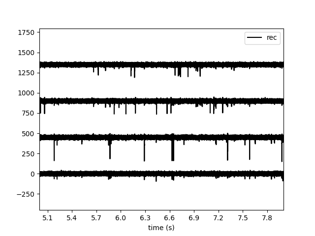
We can select time range

w_ts1 = sw.plot_timeseries(recording, time_range=(5, 8))

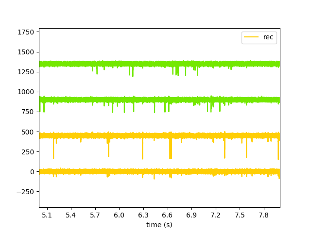
We can color with groups

recording2 = recording.clone()
recording2.set_channel_groups(channel_ids=recording.get_channel_ids(), groups=[0, 0, 1, 1])
w_ts2 = sw.plot_timeseries(recording2, time_range=(5, 8), color_groups=True)

Note: each function returns a widget object, which allows to access the figure and axis.

w_ts.figure.suptitle("Recording by group")
w_ts.ax.set_ylabel("Channel_ids")

Text(26.847222222222214, 0.5, 'Channel_ids')

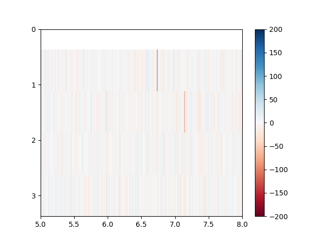
We can also use the ‘map’ mode useful for high channel count

w_ts = sw.plot_timeseries(recording, mode='map', time_range=(5, 8),
        show_channel_ids=True, order_channel_by_depth=True)

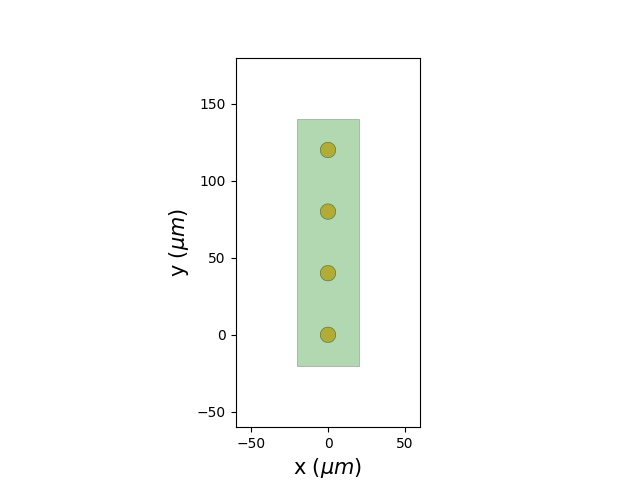
plot_electrode_geometry()

w_el = sw.plot_probe_map(recording)


plt.show()