Peaks Widgets Gallery

Some widgets are useful before sorting and works with “peaks” given by detect_peaks() function.

They are useful to check drift before running sorters.

import matplotlib.pyplot as plt

import spikeinterface.full as si

First, let’s download a simulated dataset from the repo ‘https://gin.g-node.org/NeuralEnsemble/ephy_testing_data’

local_path = si.download_dataset(remote_path='mearec/mearec_test_10s.h5')
rec, sorting = si.read_mearec(local_path)

Lets filter and detect peak on it

from spikeinterface.sortingcomponents import detect_peaks

rec_filtred = si.bandpass_filter(rec, freq_min=300., freq_max=6000., margin_ms=5.0)
print(rec_filtred)
peaks = detect_peaks(
        rec_filtred, method='locally_exclusive',
        peak_sign='neg', detect_threshold=6, n_shifts=7,
        local_radius_um=100,
        noise_levels=None,
        random_chunk_kwargs={},
        chunk_memory='10M', n_jobs=1, progress_bar=True)

Out:

BandpassFilterRecording: 32 channels - 1 segments - 32.0kHz - 10.000s

detect peaks:   0%|          | 0/5 [00:00<?, ?it/s]
detect peaks:  20%|##        | 1/5 [00:01<00:06,  1.52s/it]
detect peaks:  40%|####      | 2/5 [00:01<00:02,  1.37it/s]
detect peaks:  60%|######    | 3/5 [00:01<00:00,  2.11it/s]
detect peaks:  80%|########  | 4/5 [00:02<00:00,  2.83it/s]
detect peaks: 100%|##########| 5/5 [00:02<00:00,  2.43it/s]

peaks is a numpy 1D array with structured dtype that contains several fields:

sample_ind/channel_ind/amplitude/segment_ind

print(peaks.dtype)
print(peaks.shape)
print(peaks.dtype.fields.keys())

Out:

[('sample_ind', '<i8'), ('channel_ind', '<i8'), ('amplitude', '<f8'), ('segment_ind', '<i8')]
(796,)
dict_keys(['sample_ind', 'channel_ind', 'amplitude', 'segment_ind'])

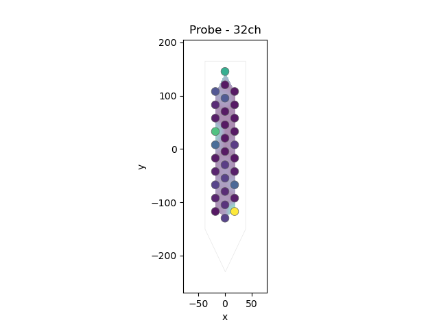
This “peaks” vector can be used in several widgets, for instance

plot_peak_activity_map()

si.plot_peak_activity_map(rec_filtred, peaks=peaks)

Out:

<spikeinterface.widgets.activity.PeakActivityMapWidget object at 0x7f0158ec9eb0>

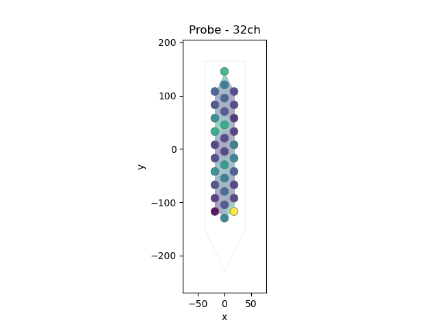
can be also animated with bin_duration_s=1.

si.plot_peak_activity_map(rec_filtred, bin_duration_s=1.)

Out:

<spikeinterface.widgets.activity.PeakActivityMapWidget object at 0x7f0158084970>

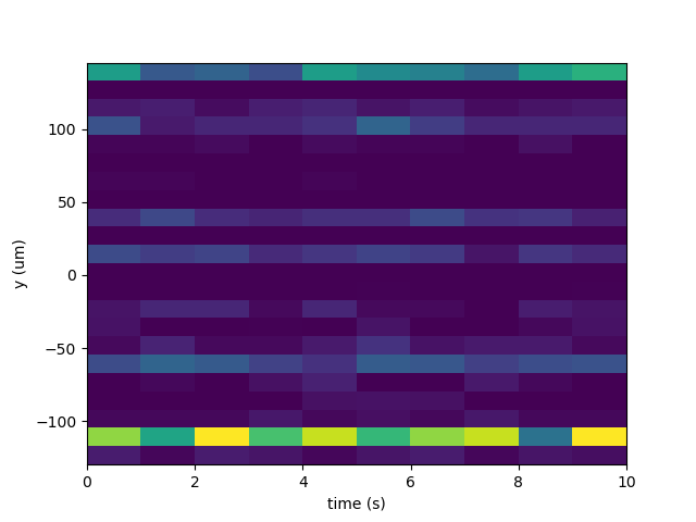
plot_drift_over_time’()

heatmap mode here bin_duration_s=1. because the rec is short (10s). a better value could 60s

si.plot_drift_over_time(rec_filtred, peaks=peaks, bin_duration_s=1.,
        weight_with_amplitudes=True, mode='heatmap')

Out:

<spikeinterface.widgets.drift.DriftOverTimeWidget object at 0x7f0158e88580>

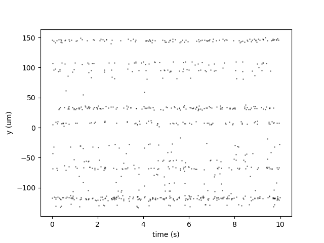
plot_drift_over_time’()

in scatter mode

si.plot_drift_over_time(rec_filtred, peaks=peaks, weight_with_amplitudes=False, mode='scatter')


plt.show()