Preprocessing Tutorial

Before spike sorting, you may need to preproccess your signals in order to improve the spike sorting performance. You can do that in SpikeInterface using the toolkit.preprocessing submodule.

import numpy as np
import matplotlib.pylab as plt
import scipy.signal

import spikeinterface.extractors as se
import spikeinterface.toolkit as st

First, let’s create a toy example:

recording, sorting = se.toy_example(num_channels=4, duration=10, seed=0)

Apply filters

Now apply a bandpass filter and a notch filter (separately) to the recording extractor. Filters are also RecordingExtractor objects. Note that theses operation are lazy the computation is done on the fly with rec.get_traces()

recording_bp = st.preprocessing.bandpass_filter(recording, freq_min=300, freq_max=6000)
print(recording_bp)
recording_notch = st.preprocessing.notch_filter(recording, freq=2000, q=30)
print(recording_notch)

Out:

BandpassFilterRecording: 4 channels - 2 segments - 30.0kHz - 20.000s
NotchFilterRecording: 4 channels - 2 segments - 30.0kHz - 20.000s

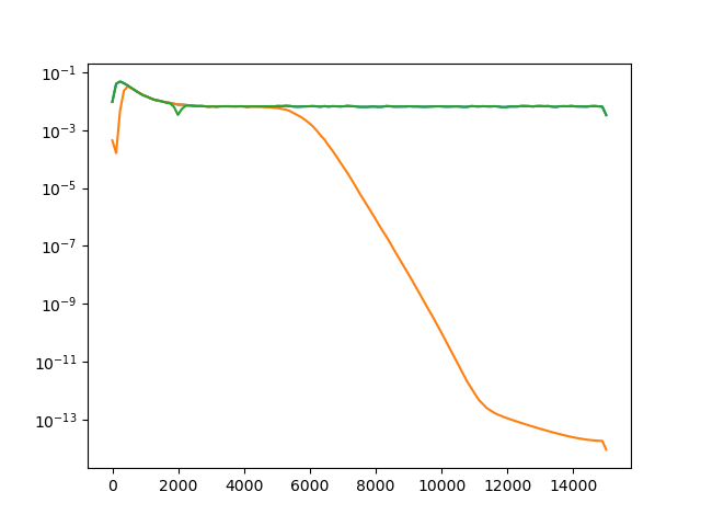
Now let’s plot the power spectrum of non-filtered, bandpass filtered, and notch filtered recordings.

fs = recording.get_sampling_frequency()

f_raw, p_raw = scipy.signal.welch(recording.get_traces(segment_index=0)[:, 0], fs=fs)
f_bp, p_bp = scipy.signal.welch(recording_bp.get_traces(segment_index=0)[:, 0], fs=fs)
f_notch, p_notch = scipy.signal.welch(recording_notch.get_traces(segment_index=0)[:, 0], fs=fs)

fig, ax = plt.subplots()
ax.semilogy(f_raw, p_raw, f_bp, p_bp, f_notch, p_notch)

Out:

[<matplotlib.lines.Line2D object at 0x7f0158cdfac0>, <matplotlib.lines.Line2D object at 0x7f0158cdf0a0>, <matplotlib.lines.Line2D object at 0x7f0158cdf700>]

Compute LFP and MUA

Local field potentials (LFP) are low frequency components of the extracellular recordings. Multi-unit activity (MUA) are rectified and low-pass filtered recordings showing the diffuse spiking activity.

In spiketoolkit, LFP and MUA can be extracted combining the bandpass_filter, rectify and resample functions. In this example LFP and MUA are resampled at 1000 Hz.

recording_lfp = st.preprocessing.bandpass_filter(recording, freq_min=1, freq_max=300)
# TODO alessio, this is for you
# recording_lfp = st.preprocessing.resample(recording_lfp, 1000)
# recording_mua = st.preprocessing.resample(st.preprocessing.rectify(recording), 1000)

The toy example data are only contain high frequency components, but  these lines of code will work on experimental data

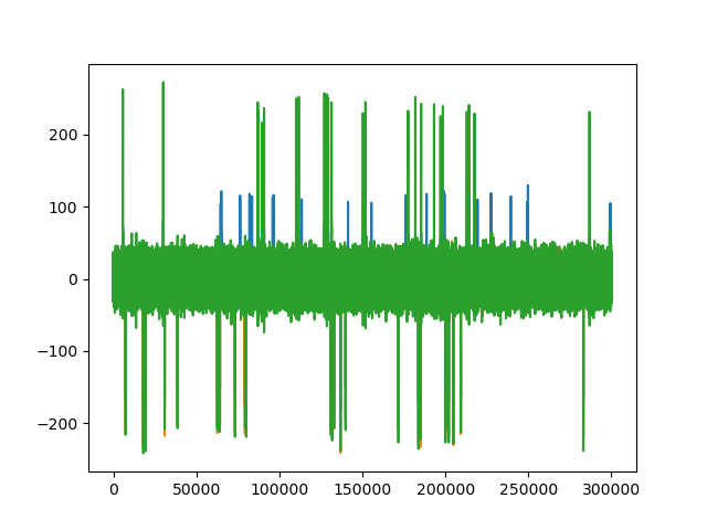
Change reference

In many cases, before spike sorting, it is wise to re-reference the signals to reduce the common-mode noise from the recordings.

To re-reference in spiketoolkit you can use the common_reference function. Both common average reference (CAR) and common median reference (CMR) can be applied. Moreover, the average/median can be computed on different groups. Single channels can also be used as reference.

recording_car = st.common_reference(recording, reference='global', operator='average')
recording_cmr = st.common_reference(recording, reference='global', operator='median')
recording_single = st.common_reference(recording, reference='single', ref_channels=[1])
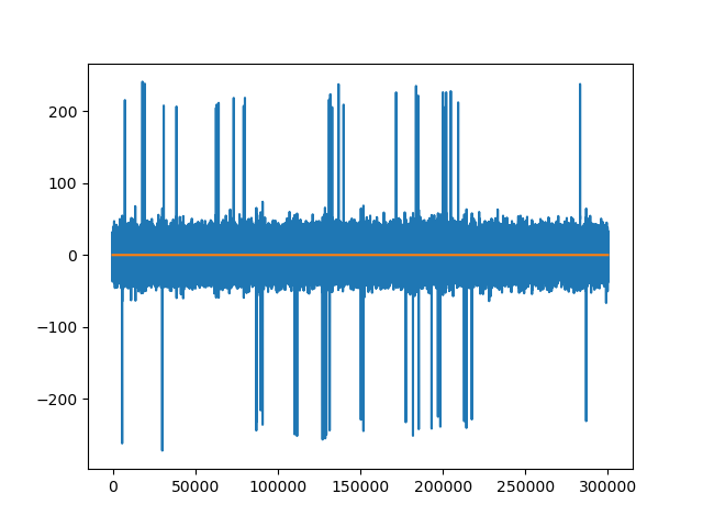
recording_single_groups = st.common_reference(recording, reference='single',
                                                            groups=[[0, 1], [2, 3]], ref_channels=[0, 2])


trace0_car = recording_car.get_traces(segment_index=0)[:, 0]
trace0_cmr = recording_cmr.get_traces(segment_index=0)[:, 0]
trace0_single = recording_single.get_traces(segment_index=0)[:, 0]
fig1, ax1 = plt.subplots()
ax1.plot(trace0_car)
ax1.plot(trace0_cmr)
ax1.plot(trace0_single)

trace1_groups = recording_single_groups.get_traces(segment_index=0)[:, 1]
trace0_groups = recording_single_groups.get_traces(segment_index=0)[:, 0]
fig2, ax2 = plt.subplots()
ax2.plot(trace1_groups)  # not zero
ax2.plot(trace0_groups)

• 
• 

Out:

[<matplotlib.lines.Line2D object at 0x7f01504c6d30>]

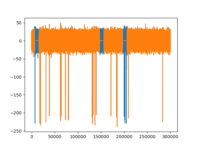
Remove stimulation artifacts

In some applications, electrodes are used to electrically stimulate the tissue, generating a large artifact. In spiketoolkit, the artifact can be zeroed-out using the remove_artifact function.

# create dummy stimulation triggers per segment
stimulation_trigger_frames = [
        [10000, 150000, 200000],
        [20000, 30000],
    ]


# large ms_before and s_after are used for plotting only
recording_rm_artifact = st.remove_artifacts(recording, stimulation_trigger_frames,
                                                         ms_before=100, ms_after=200)

trace0 = recording.get_traces(segment_index=0)[:, 0]
trace0_rm = recording_rm_artifact.get_traces(segment_index=0)[:, 0]
fig3, ax3 = plt.subplots()
ax3.plot(trace0)
ax3.plot(trace0_rm)

Out:

[<matplotlib.lines.Line2D object at 0x7f0158f1b250>]

You can list the available preprocessors with:

from pprint import pprint
pprint(st.preprocesser_dict)


plt.show()

Out:

{'bandpass_filter': <class 'spikeinterface.toolkit.preprocessing.filter.BandpassFilterRecording'>,
 'blank_staturation': <class 'spikeinterface.toolkit.preprocessing.clip.BlankSaturationRecording'>,
 'center': <class 'spikeinterface.toolkit.preprocessing.normalize_scale.CenterRecording'>,
 'common_reference': <class 'spikeinterface.toolkit.preprocessing.common_reference.CommonReferenceRecording'>,
 'filter': <class 'spikeinterface.toolkit.preprocessing.filter.FilterRecording'>,
 'normalize_by_quantile': <class 'spikeinterface.toolkit.preprocessing.normalize_scale.NormalizeByQuantileRecording'>,
 'notch_filter': <class 'spikeinterface.toolkit.preprocessing.filter.NotchFilterRecording'>,
 'rectify': <class 'spikeinterface.toolkit.preprocessing.rectify.RectifyRecording'>,
 'remove_artifacts': <class 'spikeinterface.toolkit.preprocessing.remove_artifacts.RemoveArtifactsRecording'>,
 'remove_bad_channels': <class 'spikeinterface.toolkit.preprocessing.remove_bad_channels.RemoveBadChannelsRecording'>,
 'scale': <class 'spikeinterface.toolkit.preprocessing.normalize_scale.ScaleRecording'>,
 'whiten': <class 'spikeinterface.toolkit.preprocessing.whiten.WhitenRecording'>}