Postprocessing Tutorial

Spike sorters generally output a set of units with corresponding spike trains. The toolkit.postprocessing submodule allows to combine the RecordingExtractor and the sorted SortingExtractor objects to perform further postprocessing.

import matplotlib.pylab as plt

import spikeinterface.extractors as se
import spikeinterface.toolkit as st

First, let’s create a toy example:

recording, sorting = se.example_datasets.toy_example(num_channels=4, duration=10, seed=0)

Assuming the sorting is the output of a spike sorter, the postprocessing module allows to extract all relevant information from the paired recording-sorting.

Compute spike waveforms

Waveforms are extracted with the get_unit_waveforms function by extracting snippets of the recordings when spikes are detected. When waveforms are extracted, the can be loaded in the SortingExtractor object as features. The ms before and after the spike event can be chosen. Waveforms are returned as a list of np.arrays (n_spikes, n_channels, n_points)

wf = st.postprocessing.get_unit_waveforms(recording, sorting, ms_before=1, ms_after=2,
                                          save_as_features=True, verbose=True)

Out:

Number of chunks: 1 - Number of jobs: 1

Extracting waveforms in chunks:   0%|          | 0/1 [00:00<?, ?it/s]
Extracting waveforms in chunks: 100%|##########| 1/1 [00:00<00:00, 272.32it/s]

Now waveforms is a unit spike feature!

print(sorting.get_shared_unit_spike_feature_names())
print(wf[0].shape)

Out:

['waveforms', 'waveforms_idxs']
(22, 4, 90)

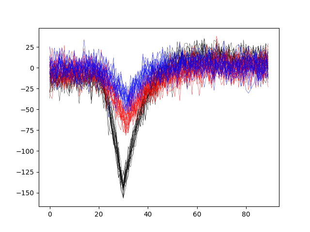
plotting waveforms of units 0,1,2 on channel 0

fig, ax = plt.subplots()
ax.plot(wf[0][:, 0, :].T, color='k', lw=0.3)
ax.plot(wf[1][:, 0, :].T, color='r', lw=0.3)
ax.plot(wf[2][:, 0, :].T, color='b', lw=0.3)

Out:

[<matplotlib.lines.Line2D object at 0x7f3e05737550>, <matplotlib.lines.Line2D object at 0x7f3e057379b0>, <matplotlib.lines.Line2D object at 0x7f3e05737c50>, <matplotlib.lines.Line2D object at 0x7f3e05737278>, <matplotlib.lines.Line2D object at 0x7f3e057370f0>, <matplotlib.lines.Line2D object at 0x7f3e05737748>, <matplotlib.lines.Line2D object at 0x7f3e05737fd0>, <matplotlib.lines.Line2D object at 0x7f3e05737978>, <matplotlib.lines.Line2D object at 0x7f3e05737400>, <matplotlib.lines.Line2D object at 0x7f3e059fa5c0>, <matplotlib.lines.Line2D object at 0x7f3e059fa240>, <matplotlib.lines.Line2D object at 0x7f3e059fab70>, <matplotlib.lines.Line2D object at 0x7f3e05886f60>, <matplotlib.lines.Line2D object at 0x7f3e05886710>, <matplotlib.lines.Line2D object at 0x7f3e05886080>, <matplotlib.lines.Line2D object at 0x7f3e05886860>, <matplotlib.lines.Line2D object at 0x7f3e058864e0>, <matplotlib.lines.Line2D object at 0x7f3e05886ac8>, <matplotlib.lines.Line2D object at 0x7f3e05886160>, <matplotlib.lines.Line2D object at 0x7f3e058869b0>, <matplotlib.lines.Line2D object at 0x7f3e058860f0>, <matplotlib.lines.Line2D object at 0x7f3e05886550>]

If the a certain property (e.g. group) is present in the  RecordingExtractor, the waveforms can be extracted only on the channels  with that property using the grouping_property and  compute_property_from_recording arguments. For example, if channel  [0,1] are in group 0 and channel [2,3] are in group 2, then if the peak  of the waveforms is in channel [0,1] it will be assigned to group 0 and  will have 2 channels and the same for group 1.

channel_groups = [[0, 1], [2, 3]]
for ch in recording.get_channel_ids():
    for gr, channel_group in enumerate(channel_groups):
        if ch in channel_group:
            recording.set_channel_property(ch, 'group', gr)
print(recording.get_channel_property(0, 'group'), recording.get_channel_property(2, 'group'))

Out:

0 1

wf_by_group = st.postprocessing.get_unit_waveforms(recording, sorting, ms_before=1, ms_after=2,
                                                   save_as_features=False, verbose=True,
                                                   grouping_property='group',
                                                   compute_property_from_recording=True)

# now waveforms will only have 2 channels
print(wf_by_group[0].shape)

Out:

(22, 4, 90)

Compute unit templates

 Similarly to waveforms, templates - average waveforms - can be easily  extracted using the get_unit_templates. When spike trains have  numerous spikes, you can set the max_spikes_per_unit to be extracted.  If waveforms have already been computed and stored as features, those  will be used. Templates can be saved as unit properties.

templates = st.postprocessing.get_unit_templates(recording, sorting, max_spikes_per_unit=200,
                                                 save_as_property=True, verbose=True)

print(sorting.get_shared_unit_property_names())

Out:

['template']

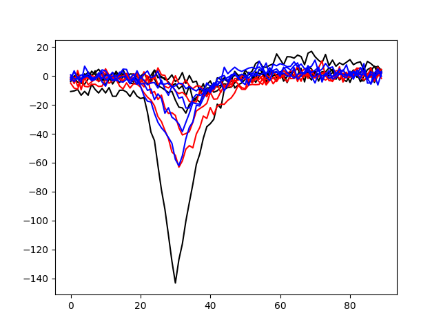
Plotting templates of units 0,1,2 on all four channels

fig, ax = plt.subplots()
ax.plot(templates[0].T, color='k')
ax.plot(templates[1].T, color='r')
ax.plot(templates[2].T, color='b')

Out:

[<matplotlib.lines.Line2D object at 0x7f3e057ac5c0>, <matplotlib.lines.Line2D object at 0x7f3e057ac710>, <matplotlib.lines.Line2D object at 0x7f3e057ac860>, <matplotlib.lines.Line2D object at 0x7f3e057ac9b0>]

Compute unit maximum channel  ——————————-

 In the same way, one can get the ecording channel with the maximum  amplitude and save it as a property.

max_chan = st.postprocessing.get_unit_max_channels(recording, sorting, save_as_property=True, verbose=True)
print(max_chan)

Out:

[0, 0, 1, 1, 1, 2, 2, 2, 3, 3]

print(sorting.get_shared_unit_property_names())

Out:

['max_channel', 'template']

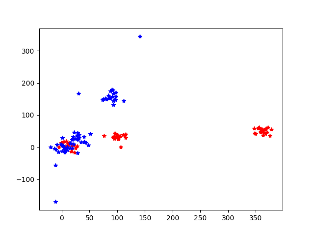
Compute pca scores  ———————

 For some applications, for example validating the spike sorting output,  PCA scores can be computed.

pca_scores = st.postprocessing.compute_unit_pca_scores(recording, sorting, n_comp=3, verbose=True)

for pc in pca_scores:
    print(pc.shape)

fig, ax = plt.subplots()
ax.plot(pca_scores[0][:, 0], pca_scores[0][:, 1], 'r*')
ax.plot(pca_scores[2][:, 0], pca_scores[2][:, 1], 'b*')

Out:

Computing waveforms
Fitting PCA of 3 dimensions on 241 waveforms
Projecting waveforms on PC
(22, 4, 3)
(26, 4, 3)
(22, 4, 3)
(25, 4, 3)
(25, 4, 3)
(27, 4, 3)
(22, 4, 3)
(22, 4, 3)
(28, 4, 3)
(22, 4, 3)

[<matplotlib.lines.Line2D object at 0x7f3e056ddda0>, <matplotlib.lines.Line2D object at 0x7f3e056dd748>, <matplotlib.lines.Line2D object at 0x7f3e056dd9b0>]

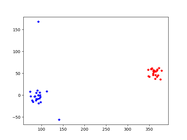
PCA scores can be also computed electrode-wise. In the previous example,  PCA was applied to the concatenation of the waveforms over channels.

pca_scores_by_electrode = st.postprocessing.compute_unit_pca_scores(recording, sorting, n_comp=3, by_electrode=True)

for pc in pca_scores_by_electrode:
    print(pc.shape)

Out:

(22, 4, 3)
(26, 4, 3)
(22, 4, 3)
(25, 4, 3)
(25, 4, 3)
(27, 4, 3)
(22, 4, 3)
(22, 4, 3)
(28, 4, 3)
(22, 4, 3)

In this case, as expected, 3 principal components are extracted for each  electrode.

fig, ax = plt.subplots()
ax.plot(pca_scores_by_electrode[0][:, 0, 0], pca_scores_by_electrode[0][:, 1, 0], 'r*')
ax.plot(pca_scores_by_electrode[2][:, 0, 0], pca_scores_by_electrode[2][:, 1, 1], 'b*')

Out:

[<matplotlib.lines.Line2D object at 0x7f3e04498e48>]

Export sorted data to Phy for manual curation

 Finally, it is common to visualize and manually curate the data after  spike sorting. In order to do so, we interface wiht the Phy  (https://phy-contrib.readthedocs.io/en/latest/template-gui/).

 First, we need to export the data to the phy format:

st.postprocessing.export_to_phy(recording, sorting, output_folder='phy', verbose=True)

Out:

Converting to Phy format
Saving files
Saved phy format to:  /home/docs/checkouts/readthedocs.org/user_builds/spikeinterface/checkouts/0.13.0/examples/modules/toolkit/phy
Run:

phy template-gui  /home/docs/checkouts/readthedocs.org/user_builds/spikeinterface/checkouts/0.13.0/examples/modules/toolkit/phy/params.py

To run phy you can then run (from terminal):  phy template-gui phy/params.py

 Or from a notebook:  !phy template-gui phy/params.py

 After manual curation you can load back the curated data using the PhySortingExtractor: