Generation module
The spikeinterface.generation module provides functions to generate recordings containing spikes,
which can be used as “ground-truth” for benchmarking spike sorting algorithms.
There are several approaches to generating such recordings. One possibility is to generate purely synthetic recordings. Another approach is to use real recordings and add synthetic spikes to them, to make “hybrid” recordings. The advantage of the former is that the ground-truth is known exactly, which is useful for benchmarking. The advantage of the latter is that the spikes are added to real noise, which can be more realistic.
For hybrid recordings, the main challenge is to generate realistic spike templates. We therefore built an open database of templates that we have constructed from the International Brain Laboratory - Brain Wide Map (available on DANDI). You can check out this collection of over 600 templates from this web app.
The spikeinterface.generation module offers tools to interact with this database to select and download templates,
manipulating (e.g. rescaling and relocating them), and construct hybrid recordings with them.
Importantly, recordings from long-shank probes, such as Neuropixels, usually experience drifts.
Such drifts can be taken into account in order to smoothly inject spikes into the recording.
The spikeinterface.generation also includes functions to generate different kinds of drift signals and drifting
recordings, as well as generating synthetic noise profiles of various types.
Some of the generation functions are defined in the spikeinterface.core.generate module, but also exposed at the
spikeinterface.generation level for convenience.
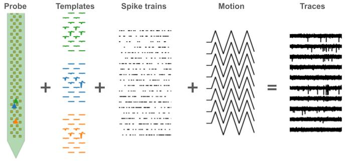
Synthetic recordings
The top level function is generate_drifting_recording().
This function generates both a static recording and a drifting recording with
exactly the same units and spikes.
The module handles many details:
any probe layout available in
probeinterface.many possible motion vectors (zigzag, bumps, random_walk) or combination of them.
non-rigid drift, the motion vector is handled at the level of the units.
control on units’ location : ‘uniform’ or ‘by layer’ (aka multi modal).
templates are generated step by step (typically 1um) along the motion axis using simple spatial rules.
templates shape are quite simple but can be controlled by many parameters (spheric/elliptical, time dynamic, spatial propagation).
spike trains have a Poisson-like distribution but can optionally be externally given by the user.
there are helper functions to inject overly synchronous spikes.
noise has a Gaussian distribution with an optional covariance using noise spatial decay.
The static and drifting recording are ‘lazy’ : traces are generated on the fly (aka on demand). The only computation is the generation of the templates which is performed at the start.
Parameters (firing, templates, locations, …) can be controlled using ranges of values or can be explicitly given unit by unit.
All parameters are carefully seeded to ensure reproducibility (at least on the same system and NumPy version).
The simplest way to generate a synthetic recording is:
import spikeinterface.full as si

rec_static, rec_drifting, gt_sorting, extra_infos = si.generate_drifting_recording(
    probe_name="Neuropixels1-128",
    num_units=200,
    duration=300.,
    seed=2205,
    extra_outputs=True,
)
Note the 4 outputs: the 2 recordings (static and drifting), the ground-truth sorting and a dictionary with more outputs (unit motion, unit position, templates, …)
But for finer control of the outputs one can input additional optional parameters:
rec_static, rec_drifting, gt_sorting, extra_infos = generate_drifting_recording(
    num_units=250,
    duration=600.0,
    sampling_frequency=30000.0,
    probe_name="Neuropixels1-384",
    # here we want a multimodal aka multi layers
    generate_unit_locations_kwargs=dict(
        margin_um=20.0,
        minimum_z=5.0,
        maximum_z=45.0,
        minimum_distance=18.0,
        max_iteration=100,
        distance_strict=False,
        distribution="multimodal",
        num_modes=3,
    ),
    # here we want to combine zizag (with a gradient in space) and bumps motion vector
    generate_displacement_vector_kwargs=dict(
        displacement_sampling_frequency=5.0,
        drift_start_um=[0, 30],
        drift_stop_um=[0, -30],
        drift_step_um=1,
        motion_list=[
            dict(
                drift_mode="zigzag",
                non_rigid_gradient=0.5,
                t_start_drift=60.0,
                t_end_drift=None,
                period_s=200,
                amplitude_factor=.5,
            ),
            dict(
                drift_mode="bumps",
                non_rigid_gradient=None,
                t_start_drift=60.0,
                t_end_drift=None,
                bump_interval_s=(30, 90.0),
                amplitude_factor=.5,
            ),
        ],
    ),
    # here we can control the parameters of the templates using ranges
    # many more parameters are available like : depolarization_ms, repolarization_ms, recovery_ms
    # positive_amplitude, smooth_ms, propagation_speed, and ellipsoid orientation...
    generate_templates_kwargs=dict(
        ms_before=1.5,
        ms_after=3.0,
        mode="ellipsoid",
        unit_params=dict(
            alpha=(150.0, 500.0),
            spatial_decay=(10, 45),
        ),
    ),
    # control the firing of the spiketrains
    generate_sorting_kwargs=dict(firing_rates=(2.0, 8.0), refractory_period_ms=4.0),
    # control the noise and covariance (spatial_decay)
    generate_noise_kwargs=dict(noise_levels=(12.0, 15.0), spatial_decay=25.0),
    # give (or not) the extra_infos dictionary
    extra_outputs=True,
    # and of course the seed :
    #  * if no idea and want to mimic geeks put 42
    #  * if you are more ego centric put your birthday
    #  * if you recently became parent put the birthday of your child
    seed=2205,
)

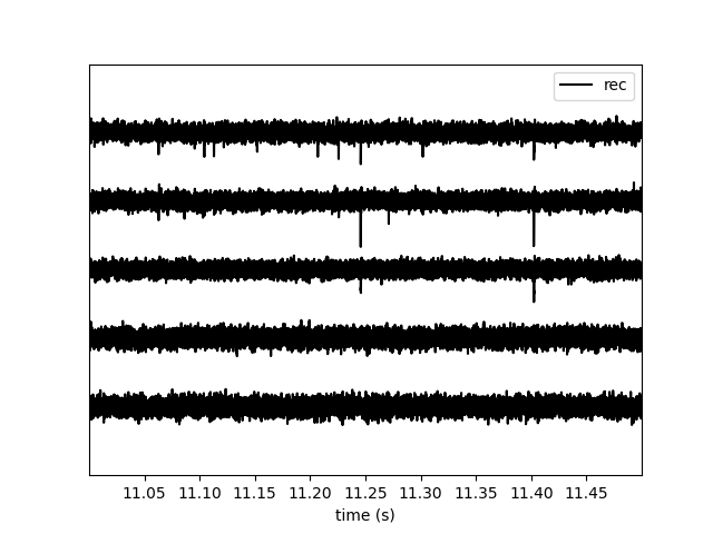
si.plot_traces(rec_static, channel_ids=rec_static.channel_ids[10:15], time_range=(11, 11.5))
The generated traces can look a bit toyish, but this generation module has proven to be very useful to the development sortingcomponents module.
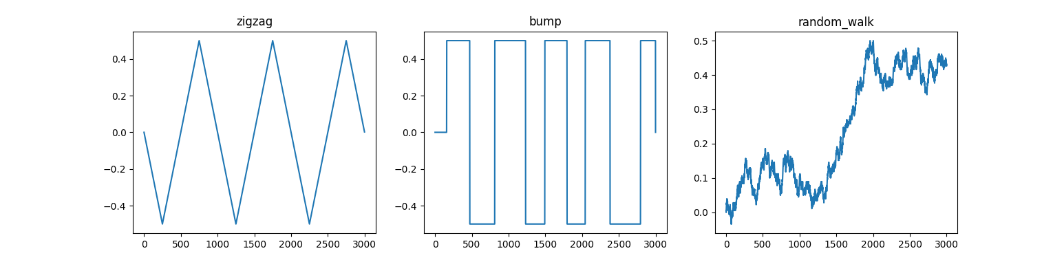
Control the drift vector
In this example we inject different drift modes to see how they influence the final motion vectors.
import matplotlib.pyplot as plt
from spikeinterface.generation import make_one_displacement_vector
fig, axs = plt.subplots(ncols=3)
for i, drift_mode in enumerate(["zigzag", "bump", "random_walk"]):
    ax = axs[i]
    motion_vector = make_one_displacement_vector(drift_mode=drift_mode, duration=600.0)
    ax.plot(motion_vector)
    ax.set_title(drift_mode)
Intersession drift
Probe drift can also happen between recording sessions. In the context of an experiment that attempts to track the activity of units across multiple sessions, changes in the position of neurons relative to the probe can create issues when trying to match units across sessions (unit-matching), and create sharp discontinuities if recordings are concatenated.
The generate_session_displacement_recordings function simulates inter-session drift by generating recording
sessions with unit positions offset. This is achieved by first generating a canonical set of unit positions,
then shifting these locations across sessions prior to injecting the resulting spikes into background noise for each session.
The full function signature is shown below:
def generate_session_displacement_recordings(
    num_units=250,
    recording_durations=(10, 10, 10),
    recording_shifts=((0, 0), (0, 25), (0, 50)),
    non_rigid_gradient=None,
    recording_amplitude_scalings=None,
    shift_units_outside_probe=False,
    sampling_frequency=30000.0,
    probe_name="Neuropixels1-128",
    generate_probe_kwargs=None,
    generate_unit_locations_kwargs=dict(
        margin_um=20.0,
        minimum_z=5.0,
        maximum_z=45.0,
        minimum_distance=18.0,
        max_iteration=100,
        distance_strict=False,
    ),
    generate_templates_kwargs=dict(
        ms_before=1.5,
        ms_after=3.0,
        mode="ellipsoid",
        unit_params=dict(
            alpha=(150.0, 500.0),
            spatial_decay=(10, 45),
        ),
    ),
    generate_sorting_kwargs=dict(firing_rates=(2.0, 8.0), refractory_period_ms=4.0),
    generate_noise_kwargs=dict(noise_levels=(12.0, 15.0), spatial_decay=25.0),
    extra_outputs=False,
    seed=None,
):
Any number of sessions can be generated by specifying the recording length and inter-session shifts
with recording_durations and recording_shifts. recording_durations gives
one duration in seconds per recording, and recording_shifts gives one
(x, y) displacement in micrometres per recording. Each tuple is relative
to the original, randomly generated unit positions. For example, it is useful to
set the first session displacement as (0, 0), in which case the unit
positions will be the initial, randomly generated positions. Then, all subsequent
positions can be interpreted as shifts relative to the first session. Typically,
only the y-axis shift is used to simulate the much more commonly corrected y-axis drift.
Estimation of inter-session drift is complicated by the fact that the signal
from units may drop out over time. To simulate this, the recording_amplitude_scalings
can be used to scale the amplitude of units across different sessions. It takes a
dictionary containing "method" (described below) and "scalings", a 2D array
of shape (num_sessions, num_units) with one scaling factor per unit per session.
A scaling of 1 leaves the amplitude unchanged, while 0 removes the unit’s
signal from the recording. The unit and its spikes remain in the ground-truth sorting.
For example, remove the fifth unit’s signal in the second session:
import numpy as np
from spikeinterface.generation.session_displacement_generator import (
    generate_session_displacement_recordings,
)

num_units = 20
scalings = np.ones((2, num_units))
scalings[1, 4] = 0.0  # Fifth unit (zero-based index 4), second session.

recordings, sortings = generate_session_displacement_recordings(
    num_units=num_units,
    recording_durations=(10.0, 10.0),
    recording_shifts=((0, 0), (0, 25)),
    recording_amplitude_scalings={
        "method": "by_passed_order",
        "scalings": scalings,
    },
    seed=42,
)
Alternatively, we may want to silence units with the highest firing frequency
(these contribute most to activity histograms often used to correct drift, and so
when they disappear from a session’s recording it has a comparatively large effect).
To do this, we can set method to by_firing_rate. Now, the scalings must be
a (num_sessions, num_units) 2d array where the order of the units dimension is
by descending firing rate. For example, to set the most active unit in the second session
to zero we would set element (1, 0) to zero. In the below example, we use a similar
approach to set the amplitude of the 5 most active neurons to half their original amplitude:
scalings = np.ones((2, num_units))
scalings[1, :5] = 0.5  # Five highest-ranked units, second session.

recordings, sortings = generate_session_displacement_recordings(
    num_units=num_units,
    recording_durations=(10.0, 10.0),
    recording_shifts=((0, 0), (0, 25)),
    recording_amplitude_scalings={
        "method": "by_firing_rate",
        "scalings": scalings,
    },
    seed=42,
)
Another consideration is what happens to units at the y-axis boundaries of the probe when it moves up or down. At one end, units disappear from the recording, but at the other end new units are introduced. This can also affect drift estimation.
To simulate this, the shift_units_outside_probe argument can be used. Setting it
True extends the generated units, adding new units at the top and bottom of the
probe. These can then enter the recording, depending on the drift. This option
cannot currently be combined with recording_amplitude_scalings.
Other controls match general generation arguments described above, such as
non_rigid_gradient, which makes displacement non-rigid. The
generate_*_kwargs arguments for configuring the
probe, unit locations, templates, spike trains, and noise are the same as above and
are used to generate the initial unit locations, template parameters, and firing rates.