Handling probe information

In order to properly spike sort, you may need to load information related to the probe you are using. You can easily load probe information in spikeinterface.extractors module.

Here’s how!

import numpy as np
import spikeinterface.extractors as se

First, let’s create a toy example:

recording, sorting_true = se.example_datasets.toy_example(duration=10, num_channels=32, seed=0)

Probe information may be required to:

• apply a channel map
• load ‘group’ information
• load ‘location’ information
• load arbitrary information

Probe information can be loaded either using a ‘.prb’ or a ‘.csv’ file. We recommend using a ‘.prb’ file, since it allows users to load several information as once.

A ‘.prb’ file is a python dictionary. Here is the content of a sample ‘.prb’ file (eight_tetrodes.prb), that splits the channels in 8 channel groups, applies a channel map (reversing the order of each tetrode), and loads a ‘label’ for each electrode (arbitrary information):

eight_tetrodes.prb:

channel_groups = {
    # Tetrode index
    0:
        {
          'channels': [3, 2, 1, 0],
          'geometry': [[0,0], [1,0], [2,0], [3,0]],
          'label': ['t_00', 't_01', 't_02', 't_03'],
        },
    1:
        {
          'channels': [7, 6, 5, 4],
          'geometry': [[6,0], [7,0], [8,0], [9,0]],
          'label': ['t_10', 't_11', 't_12', 't_13'],
        },
    2:
        {
          'channels': [11, 10, 9, 8],
          'geometry': [[12,0], [13,0], [14,0], [15,0]],
          'label': ['t_20', 't_21', 't_22', 't_23'],
        },
    3:
        {
          'channels': [15, 14, 13, 12],
          'geometry': [[18,0], [19,0], [20,0], [21,0]],
          'label': ['t_30', 't_31', 't_32', 't_33'],
         },
    4:
        {
          'channels': [19, 18, 17, 16],
          'geometry': [[30,0], [31,0], [32,0], [33,0]],
          'label': ['t_40', 't_41', 't_42', 't_43'],
        },
    5:
        {
          'channels': [23, 22, 21, 20],
          'geometry': [[36,0], [37,0], [38,0], [39,0]],
          'label': ['t_50', 't_51', 't_52', 't_53'],
        },
    6:
        {
          'channels': [27, 26, 25, 24],
          'geometry': [[42,0], [43,0], [44,0], [45,0]],
          'label': ['t_60', 't_61', 't_62', 't_63'],
        },
    7:
        {
          'channels': [31, 30, 29, 28],
          'geometry': [[48,0], [49,0], [50,0], [51,0]],
          'label': ['t_70', 't_71', 't_72', 't_73'],
        }
    }

You can load the probe file using the load_probe_file function in the RecordingExtractor. IMPORTANT This function returns a new RecordingExtractor object:

recording_tetrodes = recording.load_probe_file(probe_file='eight_tetrodes.prb')

Now let’s check what we have loaded:

print('Channel ids:', recording_tetrodes.get_channel_ids())
print('Loaded properties', recording_tetrodes.get_shared_channel_property_names())
print('Label of channel 0:', recording_tetrodes.get_channel_property(channel_id=0, property_name='label'))

Out:

Channel ids: [3, 2, 1, 0, 7, 6, 5, 4, 11, 10, 9, 8, 15, 14, 13, 12, 19, 18, 17, 16, 23, 22, 21, 20, 27, 26, 25, 24, 31, 30, 29, 28]
Loaded properties ['gain', 'group', 'label', 'location', 'offset']
Label of channel 0: t_03

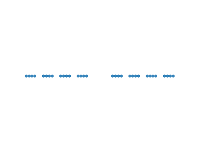
and let’s plot the probe layout:

import spikeinterface.widgets as sw
w_el_tetrode = sw.plot_electrode_geometry(recording_tetrodes)

Alternatively, one can use a ‘.csv’ file to load the electrode locations. Let’s create a ‘.csv’ file with 2D locations in a circular layout:

delta_deg = 2 * np.pi / recording.get_num_channels()
with open('circular_layout.csv', 'w') as f:
    for i in range(recording.get_num_channels()):
        angle = i * delta_deg
        radius = 50
        x = radius * np.cos(angle)
        y = radius * np.sin(angle)
        f.write(str(x) + ',' + str(y) + '\n')

When loading the probe file as a ‘.csv’ file, we can also pass a ‘channel_map’ and a ‘channel_groups’ arguments. For example, let’s reverse the channel order and split the channels in two groups:

channel_map = list(range(recording.get_num_channels()))[::-1]
channel_groups = np.array(([0] * int(recording.get_num_channels())))
channel_groups[int(recording.get_num_channels() / 2):] = 1

print('Created channel map', channel_map)
print('Created channel groups', channel_groups)

Out:

Created channel map [31, 30, 29, 28, 27, 26, 25, 24, 23, 22, 21, 20, 19, 18, 17, 16, 15, 14, 13, 12, 11, 10, 9, 8, 7, 6, 5, 4, 3, 2, 1, 0]
Created channel groups [0 0 0 0 0 0 0 0 0 0 0 0 0 0 0 0 1 1 1 1 1 1 1 1 1 1 1 1 1 1 1 1]

We can now load the probe information from the newly created ‘.csv’ file:

recording_circ = recording.load_probe_file(probe_file='circular_layout.csv',
                                           channel_map=channel_map,
                                           channel_groups=channel_groups)

Here is now the probe layout:

w_el_circ = sw.plot_electrode_geometry(recording_circ)

Let’s check that we loaded the information correctly:

print('Loaded channel ids', recording_circ.get_channel_ids())
print('Loaded channel groups', recording_circ.get_channel_groups())

Out:

Loaded channel ids [31, 30, 29, 28, 27, 26, 25, 24, 23, 22, 21, 20, 19, 18, 17, 16, 15, 14, 13, 12, 11, 10, 9, 8, 7, 6, 5, 4, 3, 2, 1, 0]
Loaded channel groups [0 0 0 0 0 0 0 0 0 0 0 0 0 0 0 0 1 1 1 1 1 1 1 1 1 1 1 1 1 1 1 1]