Getting started with SpikeInterface

In this introductory example, you will see how to use the spikeinterface to perform a full electrophysiology analysis. We will first create some simulated data, and we will then perform some pre-processing, run a couple of spike sorting algorithms, inspect and validate the results, export to Phy, and compare spike sorters.

Let’s first import the spikeinterface package. We can either import the whole package:

import spikeinterface as si

or import the different submodules separately (preferred). There are 5 modules which correspond to 5 separate packages:

• extractors : file IO and probe handling
• toolkit : processing toolkit for pre-, post-processing, validation, and automatic curation
• sorters : Python wrappers of spike sorters
• comparison : comparison of spike sorting output
• widgets : visualization

import spikeinterface.extractors as se
import spikeinterface.toolkit as st
import spikeinterface.sorters as ss
import spikeinterface.comparison as sc
import spikeinterface.widgets as sw

First, let’s create a toy example with the extractors module:

recording, sorting_true = se.example_datasets.toy_example(duration=10, num_channels=4, seed=0)

recording is a RecordingExtractor object, which extracts information about channel ids, channel locations (if present), the sampling frequency of the recording, and the extracellular traces. sorting_true is a SortingExtractor object, which contains information about spike-sorting related information, including unit ids, spike trains, etc. Since the data are simulated, sorting_true has ground-truth information of the spiking activity of each unit.

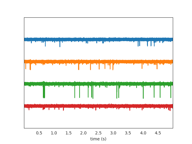
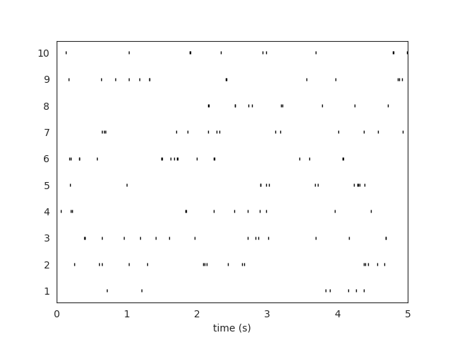
Let’s use the widgets module to visualize the traces and the raster plots.

w_ts = sw.plot_timeseries(recording, trange=[0,5])
w_rs = sw.plot_rasters(sorting_true, trange=[0,5])

• 
• 

This is how you retrieve info from a RecordingExtractor…

channel_ids = recording.get_channel_ids()
fs = recording.get_sampling_frequency()
num_chan = recording.get_num_channels()

print('Channel ids:', channel_ids)
print('Sampling frequency:', fs)
print('Number of channels:', num_chan)

Out:

Channel ids: [0, 1, 2, 3]
Sampling frequency: 30000.0
Number of channels: 4

…and a SortingExtractor

unit_ids = sorting_true.get_unit_ids()
spike_train = sorting_true.get_unit_spike_train(unit_id=unit_ids[0])

print('Unit ids:', unit_ids)
print('Spike train of first unit:', spike_train)

Out:

Unit ids: [1, 2, 3, 4, 5, 6, 7, 8, 9, 10]
Spike train of first unit: [ 21478  36186 115033 116600 124535 127993 131277 159400 163465 164645
 183164 192248 196081 214557 215749 233858 234350 250897 263249 267532
 284621 293768]

Optionally, you can load probe information using a ‘.prb’ file. For example, this is the content of custom_probe.prb:

channel_groups = {
    0: {
        'channels': [1, 0],
        'geometry': [[0, 0], [0, 1]],
        'label': ['first_channel', 'second_channel'],
    },
    1: {
        'channels': [2, 3],
        'geometry': [[3,0], [3,1]],
        'label': ['third_channel', 'fourth_channel'],
    }
}

The ‘.prb’ file uses python-dictionary syntax. With probe files you can change the order of the channels, load ‘group’ properties, ‘location’ properties (using the ‘geometry’ or ‘location’ keys, and any other arbitrary information (e.g. ‘labels’). All information can be specified as lists (same number of elements of corresponding ‘channels’ in ‘channel_group’, or dictionaries with the channel id as key and the property as value (e.g. ‘labels’: {1: ‘first_channel’, 0: ‘second_channel’})

You can load the probe file using the load_probe_file function in the RecordingExtractor. IMPORTANT: The load_probe_file function returns a *new RecordingExtractor object and it is not performed in-place:

recording_prb = recording.load_probe_file('custom_probe.prb')
print('Channel ids:', recording_prb.get_channel_ids())
print('Loaded properties', recording_prb.get_shared_channel_property_names())
print('Label of channel 0:', recording_prb.get_channel_property(channel_id=0, property_name='label'))

# 'group' and 'location' can be returned as lists:
print(recording_prb.get_channel_groups())
print(recording_prb.get_channel_locations())

Out:

Channel ids: [1, 0, 2, 3]
Loaded properties ['gain', 'group', 'label', 'location', 'offset']
Label of channel 0: second_channel
[0 0 1 1]
[[0. 0.]
 [0. 1.]
 [3. 0.]
 [3. 1.]]

Using the toolkit, you can perform pre-processing on the recordings. Each pre-processing function also returns a RecordingExtractor, which makes it easy to build pipelines. Here, we filter the recording and apply common median reference (CMR)

recording_f = st.preprocessing.bandpass_filter(recording, freq_min=300, freq_max=6000)
recording_cmr = st.preprocessing.common_reference(recording_f, reference='median')

Now you are ready to spikesort using the sorters module! Let’s first check which sorters are implemented and which are installed

print('Available sorters', ss.available_sorters())
print('Installed sorters', ss.installed_sorters())

Out:

Available sorters ['combinato', 'hdsort', 'herdingspikes', 'ironclust', 'kilosort', 'kilosort2', 'kilosort2_5', 'kilosort3', 'klusta', 'mountainsort4', 'spykingcircus', 'tridesclous', 'waveclus', 'yass']
Installed sorters ['klusta', 'mountainsort4', 'tridesclous']

The ss.installed_sorters() will list the sorters installed in the machine. We can see we have Klusta and Mountainsort4 installed. Spike sorters come with a set of parameters that users can change. The available parameters are dictionaries and can be accessed with:

print(ss.get_default_params('mountainsort4'))
print(ss.get_default_params('klusta'))

Out:

{'detect_sign': -1, 'adjacency_radius': -1, 'freq_min': 300, 'freq_max': 6000, 'filter': True, 'whiten': True, 'curation': False, 'num_workers': None, 'clip_size': 50, 'detect_threshold': 3, 'detect_interval': 10, 'noise_overlap_threshold': 0.15}
{'adjacency_radius': None, 'threshold_strong_std_factor': 5, 'threshold_weak_std_factor': 2, 'detect_sign': -1, 'extract_s_before': 16, 'extract_s_after': 32, 'n_features_per_channel': 3, 'pca_n_waveforms_max': 10000, 'num_starting_clusters': 50, 'chunk_mb': 500, 'n_jobs_bin': 1}

Let’s run mountainsort4 and change one of the parameter, the detection_threshold:

sorting_MS4 = ss.run_mountainsort4(recording=recording_cmr, detect_threshold=6)

Out:

Warning! The recording is already filtered, but Mountainsort4 filter is enabled. You can disable filters by setting 'filter' parameter to False

Alternatively we can pass full dictionary containing the parameters:

ms4_params = ss.get_default_params('mountainsort4')
ms4_params['detect_threshold'] = 4
ms4_params['curation'] = False

# parameters set by params dictionary
sorting_MS4_2 = ss.run_mountainsort4(recording=recording, **ms4_params)

Out:

Warning! The recording is already filtered, but Mountainsort4 filter is enabled. You can disable filters by setting 'filter' parameter to False

Let’s run Klusta as well, with default parameters:

sorting_KL = ss.run_klusta(recording=recording_cmr)

Out:

RUNNING SHELL SCRIPT: /home/docs/checkouts/readthedocs.org/user_builds/spikeinterface/checkouts/0.13.0/examples/getting_started/klusta_output/run_klusta.sh
/home/docs/checkouts/readthedocs.org/user_builds/spikeinterface/checkouts/0.13.0/doc/sources/spikesorters/spikesorters/basesorter.py:158: ResourceWarning: unclosed file <_io.TextIOWrapper name=6 encoding='UTF-8'>
  self._run(recording, self.output_folders[i])

The sorting_MS4 and sorting_MS4 are SortingExtractor objects. We can print the units found using:

print('Units found by Mountainsort4:', sorting_MS4.get_unit_ids())
print('Units found by Klusta:', sorting_KL.get_unit_ids())

Out:

Units found by Mountainsort4: [1, 2, 3, 4, 5, 6]
Units found by Klusta: [0, 2, 3, 4, 5, 6, 7, 8, 9, 10, 11, 12]

Once we have paired RecordingExtractor and SortingExtractor objects we can post-process, validate, and curate the results. With the toolkit.postprocessing submodule, one can, for example, get waveforms, templates, maximum channels, PCA scores, or export the data to Phy. Phy is a GUI for manual curation of the spike sorting output. To export to phy you can run:

st.postprocessing.export_to_phy(recording, sorting_KL, output_folder='phy')

Then you can run the template-gui with: phy template-gui phy/params.py and manually curate the results.

Validation of spike sorting output is very important. The toolkit.validation module implements several quality metrics to assess the goodness of sorted units. Among those, for example, are signal-to-noise ratio, ISI violation ratio, isolation distance, and many more.

snrs = st.validation.compute_snrs(sorting_KL, recording_cmr)
isi_violations = st.validation.compute_isi_violations(sorting_KL, duration_in_frames=recording_cmr.get_num_frames())
isolations = st.validation.compute_isolation_distances(sorting_KL, recording_cmr)

print('SNR', snrs)
print('ISI violation ratios', isi_violations)
print('Isolation distances', isolations)

Out:

SNR [42.46399044 65.03311047 33.47233692  4.08219477  3.85108472 15.98982149
 30.0173599  13.51226553  3.90097428 10.24819052 11.55758006  4.07045108]
ISI violation ratios [0.         0.         0.         0.54469044 0.40498685 2.60091552
 0.         7.4906367  0.39824982 2.10674157 0.         0.45861041]
Isolation distances [           nan 2.05579984e+04 1.82982173e+03 6.58686067e+00
 6.11073398e+00 1.98799187e+01 1.67309619e+03 9.72017815e+00
 8.77673461e+00 1.14200866e+01 1.31270206e+01 9.90547581e+00]

Quality metrics can be also used to automatically curate the spike sorting output. For example, you can select sorted units with a SNR above a certain threshold:

sorting_curated_snr = st.curation.threshold_snrs(sorting_KL, recording_cmr, threshold=5, threshold_sign='less')
snrs_above = st.validation.compute_snrs(sorting_curated_snr, recording_cmr)

print('Curated SNR', snrs_above)

Out:

Curated SNR [42.46399044 65.03311047 33.47233692 15.98982149 30.0173599  13.51226553
 10.24819052 11.55758006]

The final part of this tutorial deals with comparing spike sorting outputs. We can either (1) compare the spike sorting results with the ground-truth sorting sorting_true, (2) compare the output of two (Klusta and Mountainsor4), or (3) compare the output of multiple sorters:

comp_gt_KL = sc.compare_sorter_to_ground_truth(gt_sorting=sorting_true, tested_sorting=sorting_KL)
comp_KL_MS4 = sc.compare_two_sorters(sorting1=sorting_KL, sorting2=sorting_MS4)
comp_multi = sc.compare_multiple_sorters(sorting_list=[sorting_MS4, sorting_KL],
                                         name_list=['klusta', 'ms4'])

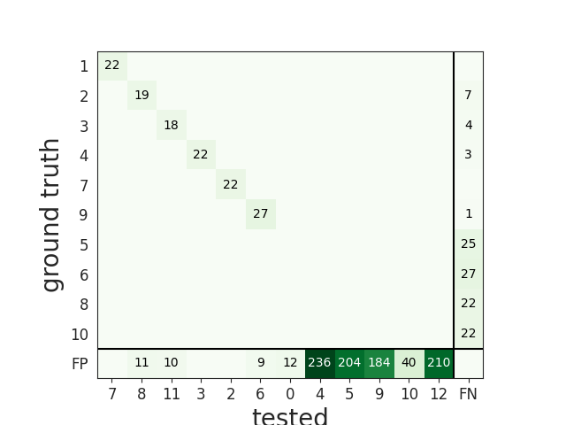
When comparing with a ground-truth sorting extractor (1), you can get the sorting performance and plot a confusion matrix

comp_gt_KL.get_performance()
w_conf = sw.plot_confusion_matrix(comp_gt_KL)

When comparing two sorters (2), we can see the matching of units between sorters. For example, this is how to extract the unit ids of Mountainsort4 (sorting2) mapped to the units of Klusta (sorting1). Units which are not mapped has -1 as unit id.

mapped_units = comp_KL_MS4.get_mapped_sorting1().get_mapped_unit_ids()

print('Klusta units:', sorting_KL.get_unit_ids())
print('Mapped Mountainsort4 units:', mapped_units)

Out:

Klusta units: [0, 2, 3, 4, 5, 6, 7, 8, 9, 10, 11, 12]
Mapped Mountainsort4 units: [-1, 5, 3, -1, -1, 6, 1, -1, -1, -1, -1, -1]

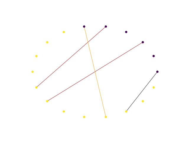
When comparing multiple sorters (3), you can extract a SortingExtractor object with units in agreement between sorters. You can also plot a graph showing how the units are matched between the sorters.

sorting_agreement = comp_multi.get_agreement_sorting(minimum_agreement_count=2)

print('Units in agreement between Klusta and Mountainsort4:', sorting_agreement.get_unit_ids())

w_multi = sw.plot_multicomp_graph(comp_multi)

Out:

Units in agreement between Klusta and Mountainsort4: [0, 2, 4, 5]